Break up! When it is time, the inevitable always happens & we have to part ways. Who is ’we’ you ask? It’s the content within the cells in MS Excel!
Not at all those within are meant to be there together. Exampli gratia, a column containing entries of City Name & its Pincode or a Client Name & their ID or Product Names & their Prices. All these entries though they may be related to each other need not necessarily be together, especially when one needs to work with that data. This calls for splitting them into separate entities & we are going to look at how that can be done.
Following is the dataset where one can find both the Client’s Name & their contact number recorded within the same cells of column C.
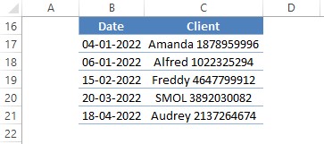
With the above data, we can’t go further with any computations involving only the contact numbers of the client or only their names. So, splitting them seems to be the only viable solution.
The solution being conjured up now, how is that we get about executing it?
ENTER TEXT TO COLUMNS!
Splitting Cells using Text to Columns:
The column whose entries are to be split is selected as shown in the following image.
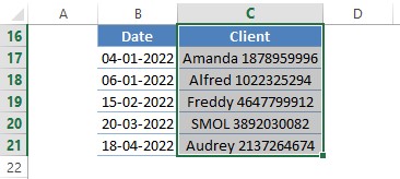
Once done, it’s time that we shift our sight to the Data Tab.
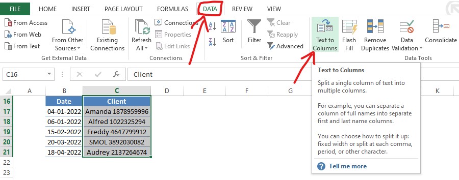
Click on the Text to Columns option as indicated in the above image. It shall make the following pop-up titled Convert Text to Columns Wizard to appear.
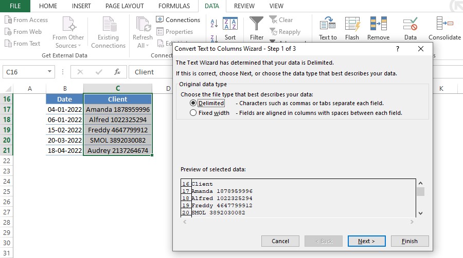
Here, there are 2 options to choose from, listed in the Convert Text to Columns Wizard & the one in which we would be interested in is the Delimited option that is selected by default. The reason is quite simple & becomes evident when one pays close attention to the description of the Delimited given in the above image.
Our job here is done & now let’s click Next.
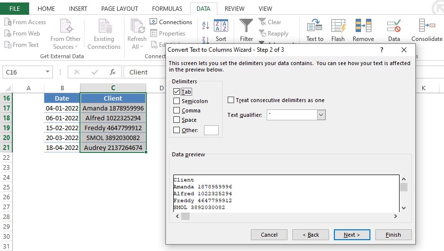
Step 2 of the Wizard welcomes us with Tab selected as a default delimiter. Change the selection to Space & an immediate change appears in the Data Preview section as shown below.
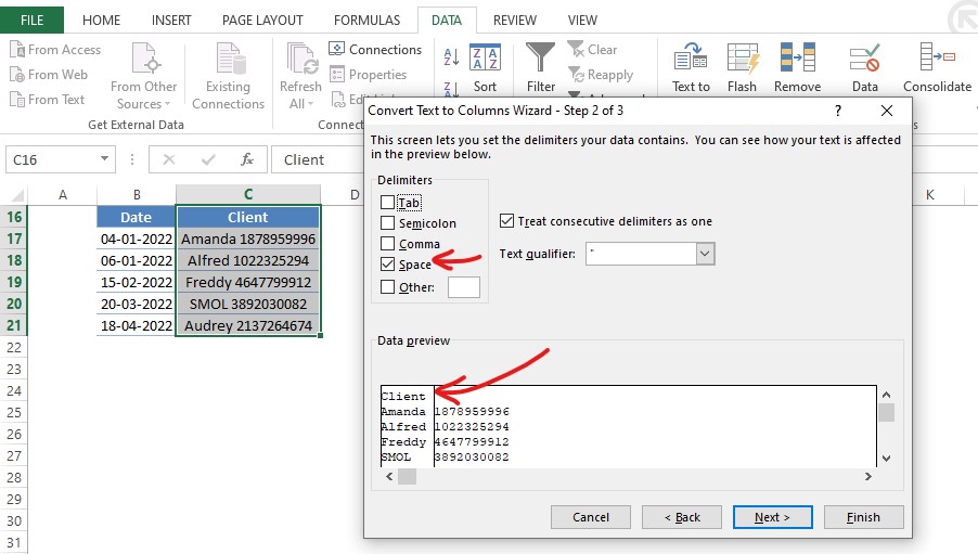
Click next & we enter the final step of this wizard. We would be prompted to choose a format for each of the columns into which the data has been split. Let us retain the format as ‘General’ for both the columns, since it would retain textual data as is & would also detect numerical data, converting them into the required format.
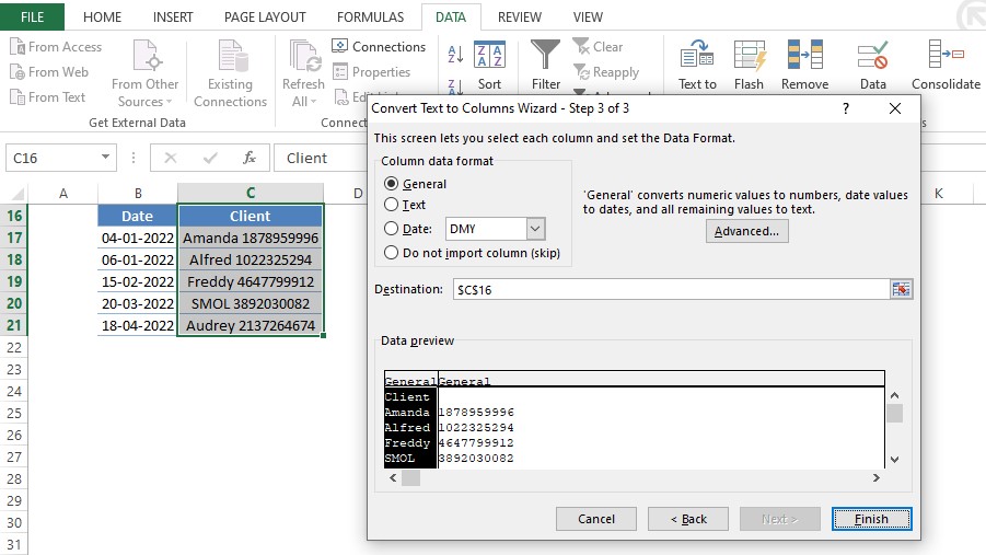
Click Finish & we are done and dusted.
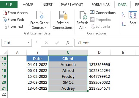
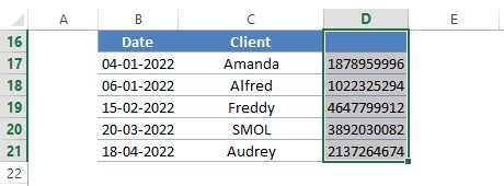
The above would be the final outcome where the names of the client have been separated from their contact numbers. One can also use the format painter option to apply the same cell formatting from column C titled Client to that of its adjacent column containing the contact numbers.
It can be done by selecting all the entries under Client as shown in the above image & clicking on the Format Painter option.
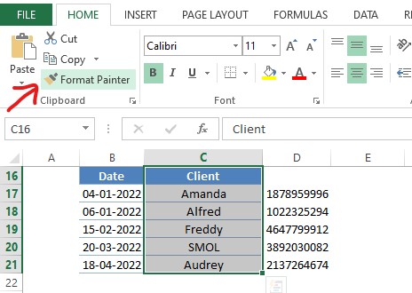
Once done, hover the cursor & click on cell D16. All entries would now appear similar in formatting to that of their adjacent column.
Conclusion:
Now we have reached the end of this article about splitting cells in MS Excel. QuickExcel has numerous other articles too that can come in handy for those who are looking for something in MS Excel. Here’s one which elaborates on how to remove blank rows in MS Excel. Ciao!
