So, you have got all the data recorded in a table categorized under different columns of your spreadsheet. You are very proud of yourself & bask in the glory of your achievement.
What possibly can go wrong? – you might think.
What if there are some blank rows in the middle to fiddle with your data. These would create discontinuities while navigating through the dataset and can also be a reason for the changes in the format which makes the last cell at the bottom look entirely different than that of the topmost cell.
In this article, we would be diving into the techniques on how to chase these blank-ers away for the greater good and to restore uniformity to our data. So, what tool are we going to pick from the arsenal of MS Excel for this very purpose?
FILTER!
The following is the table in which we would be trying to remove all those blank rows. So, let’s get filtering.
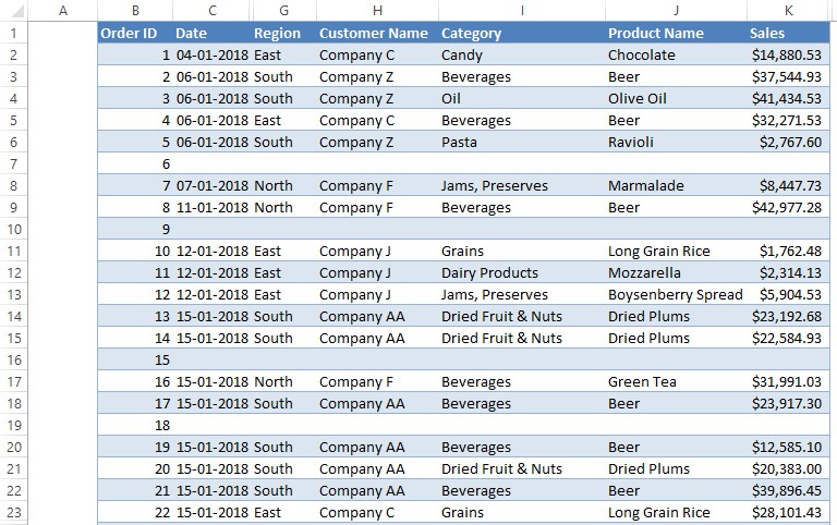
Filtering to Remove the Blank Spaces
Before moving on to the different ways how to apply a filter, we shall get done with the pre-requisite which is selecting the header row. The first row of the table containing the titles of the respective columns is selected.
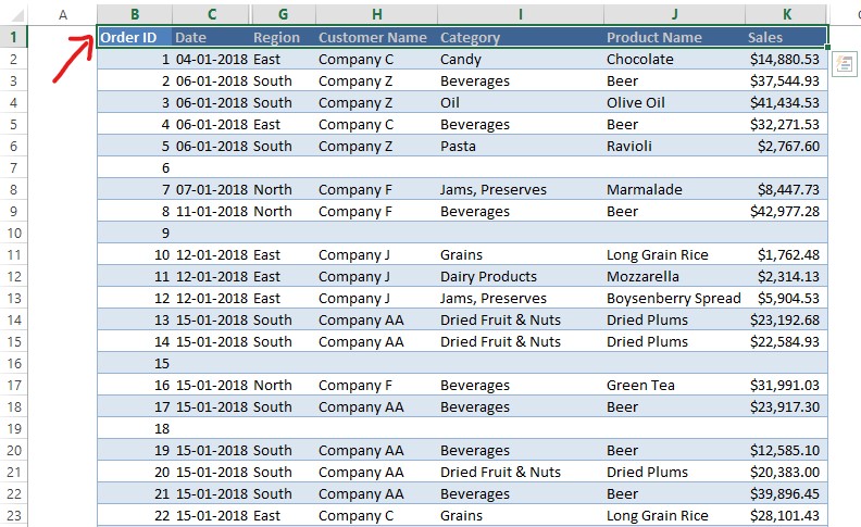
There is a list of choices presenting themselves right now for you to choose your favourite.
- Keyboard Shortcut
- Hotkey Method
- Selecting from the Home Tab
Method 1 – Keyboard Shortcut
Hit the following keys one after the other & NOT simultaneously. But the emphasis here is not to lift the fingers pressing one key when the other is being hit. To put it in simple words, one has got to press CTRL & then without lifting the finger off that key, press SHIFT & then without lifting the finger off the SHIFT key, press the letter key ‘L’ (Now, you know why we have 10 fingers).
CTRL + SHIFT + L
Once, done all the selected cells will be applied with the filters.
Method 2 – Hotkey Method
This method follows the letters that would appear on & within the Tabs when the ALT key is pressed. For applying filters, it would be,
ALT – H – S – F
Unlike the previous method, it ain’t necessary for one to keep the previous key pressed when the other keys are also pressed. Here, one can very well lift off the finger after each key is pressed.
Method 3 – Selecting from the Home Tab
Click on the option shown in the below image, to apply filters using this method.
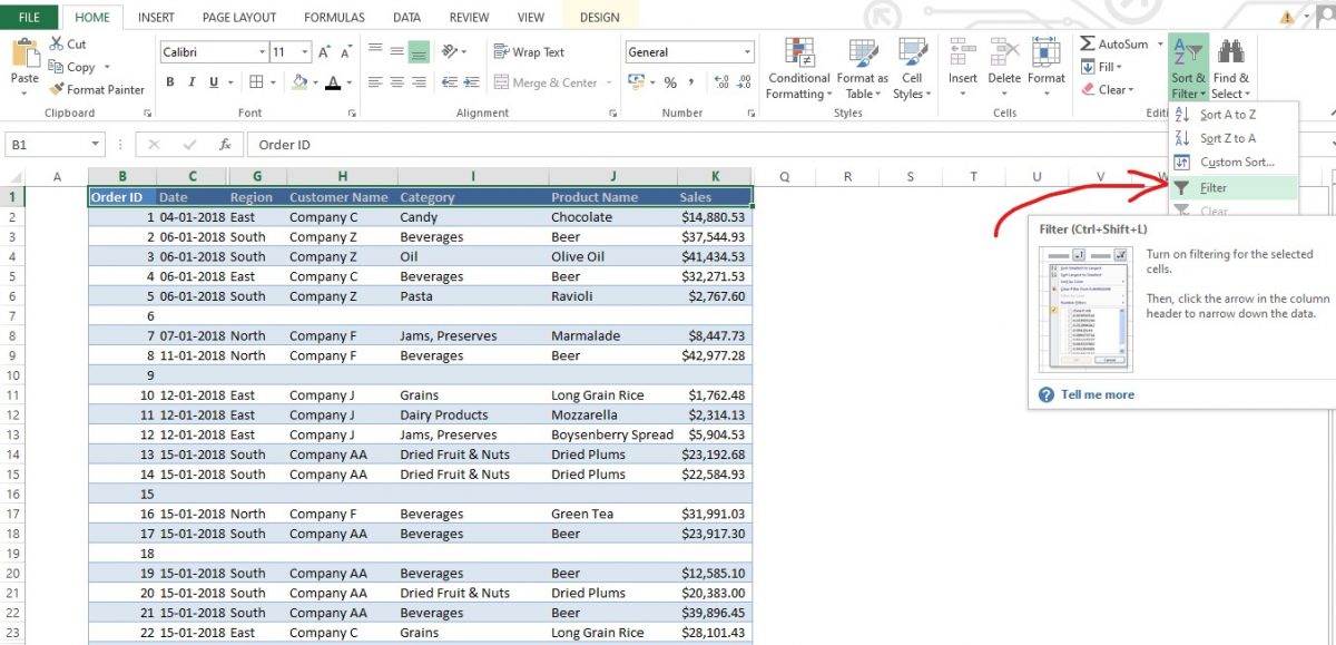
Once done, the filters would appear on the selected rows as shown in the following image.
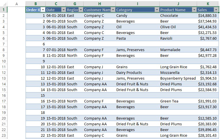
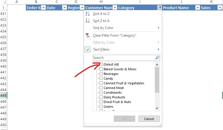
Click on any of the filters from columns C to K and a drop-down would appear just as shown below.
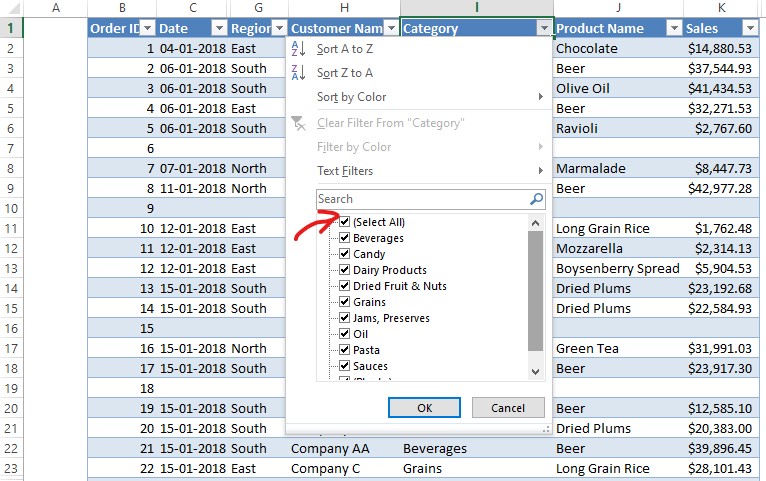
Uncheck the box named (Select All) as indicated in the above image & scroll down until you can lay your eyes on the (Blanks).
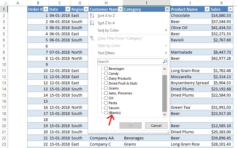
Now click on the checkbox of (Blanks) and hit OK as shown in the below image.
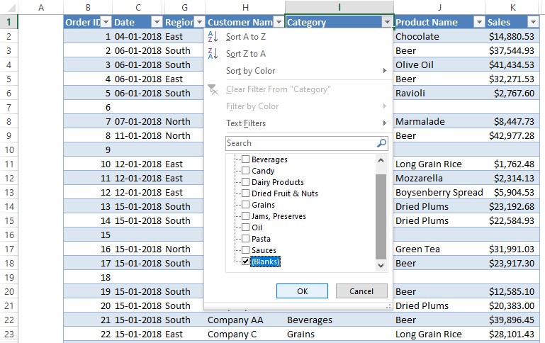
Only the blank rows would be displayed now.

Select all the rows, right click & choose delete as shown below. One can also use the keyboard shortcut of CTRL + MINUS (-) sign to delete the blank rows.
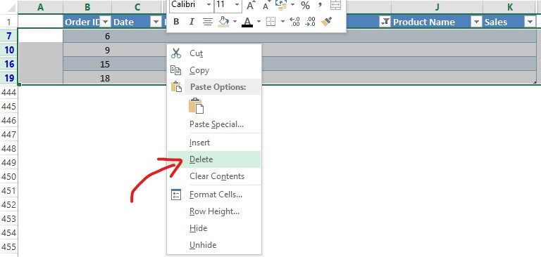
After the blank rows are deleted, reselect the (Select All) option as shown below, to clear the filter.
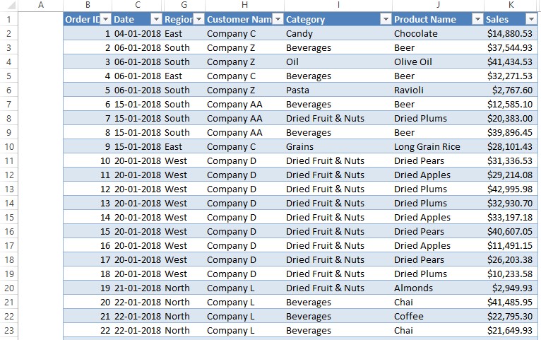
The entire tabulation removed with the blank rows would be displayed. Mission accomplished!
Conclusion
Now we have come to the end of this article. For those who are wondering how to insert a new row in MS Excel, do have a look at this article which details the different ways to do it. QuickExcel also has numerous other articles, which could help you in many ways to use MS Excel. Cheers!
