We are all searching for something in our lives, aren’t we? Sometimes we search for clues, sometimes for answers & weirdly sometimes for questions too! In this article, we will be having a look at a built-in feature of MS Excel that helps us to search for things within the spreadsheet.
The name VLOOKUP might ring a bell even for an amateur MS Excel user, but HLOOKUP won’t bring the same effect. It is something that is rarely tapped into by users. Nevertheless, we would be exploring the different ways of putting it to use in the following sections.
Also read: What is VLOOKUP and How to Use VLOOKUP in Excel?
The letter ‘V’ in the VLOOKUP stands for vertical indicating that the search term would be looked up in the vertical direction whilst the letter ‘H’ in the HLOOKUP stands for horizontal indicating that the search term would be looked up in the horizontal direction.
Syntax of HLOOKUP
Following is the syntax of HLOOKUP containing both the mandatory and optional constructs to make it function.
=HLOOKUP(lookup_value, table_array, row_index_num, [range_lookup])
where,
- lookup_value – the item which is to be searched elsewhere (source)
- table_array – the destination table within which the item is to be searched
- row_index_num – the row position from the start of the destination table whose value is to be returned
- [range lookup] – an optional element set to FALSE (0) by default to return the value that exactly matches the search item. In case the requirement is to get an approximate match, this can be changed to TRUE (1).
HLOOKUP for Exact Match
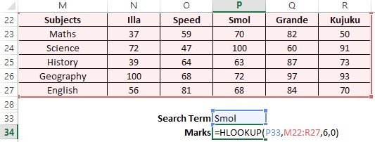
We shall try to find the exact match for the search term within the destination table array & return a specific value for the desired row in the below dataset of student scores across different subjects.

Let us get started by constructing the formula for HLOOKUP to return the marks scored by Smol in ‘English’. As always, it begins with an equals sign (=) followed by typing HLOOKUP and opening parenthesis.

Then the search term is selected as shown in the above image, followed by including a comma before selecting the table range within which the search is to be done.

It is to be noted that after each input a comma is to be provided to differentiate the inputs from each other. Now one ought to type the row number where the marks for English lie which in this case is ‘6’. Finally, the formula is completed by typing ‘0’ (zero) in the place for range_lookup as shown below.

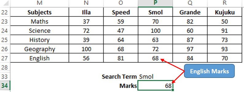
Hit ENTER once done & it will return the corresponding value of the search term.

Using Wildcard Characters in HLOOKUP
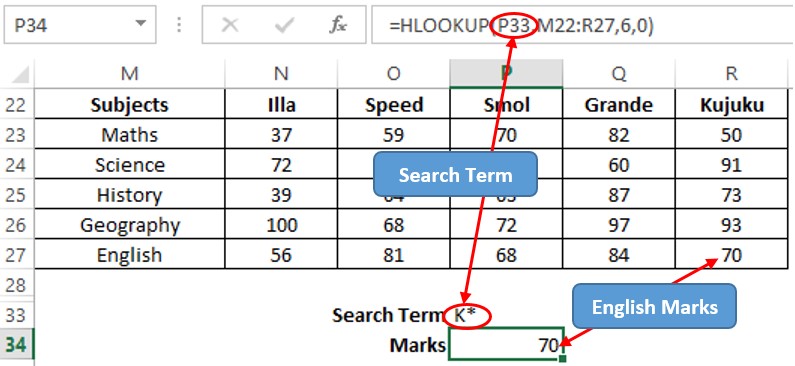
Say for instance one doesn’t know the full name but only the starting letter of a student & would like to know the marks that the student has scored in English – HLOOKUP paves way for retrieving that too!
One can type in the first letter of the name followed by an asterisk (*) to indicate the formula that the name which starts with that letter is the search term. Applying this to the dataset given earlier to find the mark in English scored by a student whose name starts with ‘K’ we get the following.

The first letter of a search term followed by an asterisk (*) is called a wildcard character and this can come in handy when one does not know the fullest search term.
Conclusion
Hope this article helped you understand the different ways of using HLOOKUP in MS Excel. Have a look at this article to know more about comparing two columns using VLOOKUP in MS Excel. There are numerous equally interesting & informative articles in QuickExcel that serve to be of great help for your path to mastering MS Excel. Until then, cheers!
