The Ultimate Guide to Sorting Data in Excel?

This article is a detailed step-by-step guide on sorting data in Excel. We will learn to sort data in Excel on the basis of date, color, alphabetically, numerically, and custom sorting.

Steps to sort columns in Excel

Let’s get started with learning to sort data in Excel with various examples below.

We have a dataset containing textual, numerical, and time data types. Let us learn to sort each type of data in Excel with the help of this example.

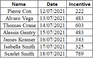
sample database 10 — Dataset with Different Types of Contents

1. Sorting data alphabetically

To alphabetically sort the data in ascending (A to Z) or descending (Z to A) order, do as follows.

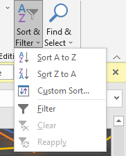
alphabet options — Sorting for Alphabets

Select a cell with textual data in its column.
Or select the entire range with textual data.
Go to the Home tab, and pull down on Sort & Filter under Editing group.
Select A to Z for ascending order or Z to A for descending order sorting of the textual data.

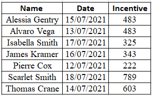
Sorting Data in Excel — Alphabets Arranged in Ascending Order

You can find that the text in the dataset has now been arranged in ascending order alphabetically.

2. Sorting data numerically

To numerically sort the data in ascending (lowest or highest) or descending (highest to lowest) order, do as follows.

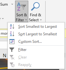
Select a cell with numerical data in its column.
Or select the entire range with numerical data.
Go to the Home tab, and pull down on Sort & Filter under Editing group.
Select Smallest to Largest for ascending order or Largest to Smallest for descending order sorting of the numerical data.

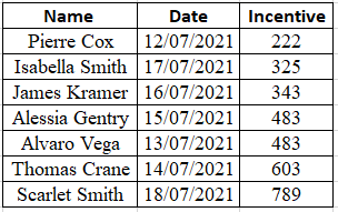
You can find that the numbers in the dataset have been arranged in ascending order.

3. Sorting data by date or time

To sort the data by date in newest to oldest or oldest to newest order, do as follows.

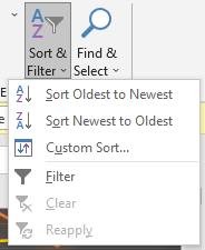
Select a cell with dates in its column.
Or select the entire range with time or date.
Go to the Home tab, and pull down on Sort & Filter under Editing group.
Select Oldest to Newest for ascending order or Newest to Oldest for descending order sorting of the dates.

sample database 11 — Dates Arranged in Oldest to Newest Order

You can find that the dates in the dataset have been arranged in oldest to newest order.

Learn more about sorting data by date here: How to sort by date in Excel?

Using Custom Sort in Excel

The custom sorting options in Excel allow you to sort data by cell color, font color, conditional formatting icons, and cell values.

1. Sorting data by cell color

You would first require to color cells in order to sort them by cell color in Excel. To color a cell in Excel.

Select the cell you want to color.
Go to the Home tab.
Under Fonts group.
Click or pull down on the paint bucket icon to fill color in the cell.

This is how colored cells look like in Excel.

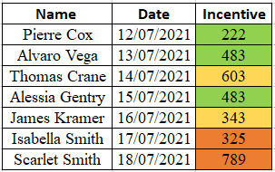
To sort data in a table by cell color, do as follows next.

Select a cell within the data range.
Go to the Home tab, and pull down on Sort & Filter under Editing group.
Select Custom Sort.
A new window named Sort opens.

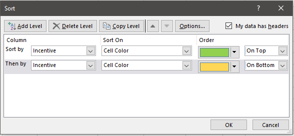
cell color sorting — Sorting by Cell Color

Select the column name you’ve applied cell colors to under Column. Here, we will choose “Incentive” as we have colored cells in this column.
Select Cell Color under Sort On.
Select color and choose if you want it to be placed at the top or bottom under Order.
Add additional levels of sorting by clicking Add Level at the top.
Set different sorting types for other cell colors in the same way.
Click OK when you’re done.

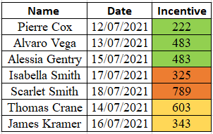
sorted cell color — Sorted by Cell Color

You can see that all green-colored cells are at the top positions and all yellow-colored cells are at the bottom positions.

2. Sorting data by font color

You would first require to color the text in order to sort them by font color in Excel.

To color text in Excel.

Select the cells with texts you want to color.
Go to the Home tab.
Under Fonts group.
Click or pull down on the A icon to add color to texts.

This is how colored texts look like in Excel.

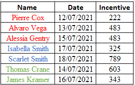
To sort data in a table by font color, do as follows next.

Select a cell within the data range.
Go to the Home tab, and pull down on Sort & Filter under Editing group.
Select Custom Sort.
A new window named Sort opens.

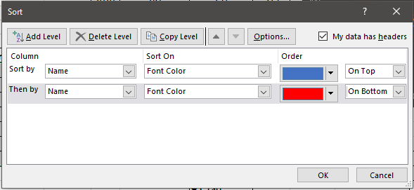
font color sorting — Sorting by Font Color

Select the column name you’ve applied cell colors to under Column. Here, we will choose “Name” as we have colored texts in this column.
Select Font Color under Sort On.
Select color and choose if you want it to be placed at the top or bottom under Order.
Add additional levels of sorting by clicking Add Level at the top.
Set different sorting types for other font colors in the same way.
Click OK when you’re done.

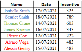
sorted font color — Sorted by Font Color

You can see that all blue-colored texts are at the top positions and all red-colored cells are at the bottom positions.

3. Sorting data by conditional formatting icons

You would first require to apply conditional formatting icons to cells in order to sort them by conditional formatting icons in Excel.

To apply conditional formatting in Excel.

Select the cells you want to apply the icons to.
Go to the Home tab.
Under Styles group, pull down on Conditional Formatting.
Pull on the Icon Sets option and choose any icon set you like.

This is what conditional formatting icons look like.

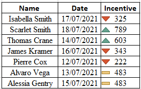
icons applied — Icons Applied via Conditional Formatting

To sort data in a table by conditional formatting, do as follows next.

Select a cell within the data range.
Go to the Home tab, and pull down on Sort & Filter under Editing group.
Select Custom Sort.
A new window named Sort opens.

Sorting by Icons

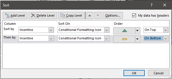
Select the column name you’ve applied cell colors to under Column. Here, we will choose “Incentive” as we have icons applied in this column.
Select Conditional Formatting Icons under Sort On.
Select an icon and choose if you want it to be placed at the top or bottom under Order.
Add additional levels of sorting by clicking Add Level in the top.
Set different sorting types for other icons in the same way.
Click OK when you’re done.

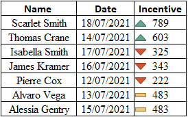
You can see that all green-colored icons are at the top positions and all yellow-colored icons are at the bottom positions.

Sorting multiple columns in Excel

Multiple columns can be sorted easily with the help of the Custom Sort tool in Excel. To sort multiple columns in Excel, follow these steps.

Select a cell in the table, go to the Home tab, and pull down on Sort & Filter under Editing group.
Select Custom Sort.
Add different kinds of sorting types for any column you like by clicking Add Level.

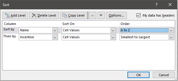
multiple column sorting — Sorting Multiple Columns

You can see that multiple columns have been sorted via custom sort in Excel.

Sorting rows in Excel

Let’s take a sample horizontal database with its headers in rows.

In order to sort rows in Excel, follow these steps.

Select a cell within the data range.
Go to the Home tab, and pull down on Sort & Filter under Editing group.
Select Custom Sort.
Click on Options at the top.

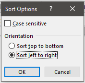
Select Sort left to right and click OK.
Select the row number for which you want to sort data.
Sort data based on font color, cell color, cell values, or conditional formatting icons.
Click OK when you’re done.

You can see that your rows have been sorted from largest to smallest numbers.

Conclusion

This article was an ultimate guide to sorting data in Excel, step-by-step. Follow these steps to learn in-depth about sorting any type of content in Microsoft Excel, all for free! Feel free to comment your doubts below.

References: Microsoft, GCF Global