Conditional formatting is used for multiple important in Microsoft Excel. Let’s discover how we can use this brilliant tool and understand how it helps us in data management.
Using Conditional Formatting in Excel
Let’s get started with this ultimate guide to using conditional formatting in Excel for different tasks.
1. Highlighting cells based on a condition
Conditional formatting can be used to highlight cells based on a variety of conditions that you can set.
You can highlight specific cells greater than, less than, or equal to a specific number. Or you could also highlight cells with duplicate values, or a specific text, or even a particular date.
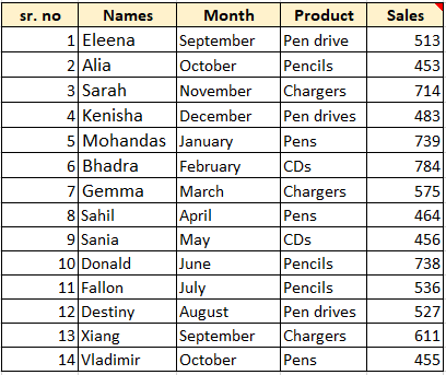
Let us see how we can use conditional formatting to highlight cells in Excel. We have taken a sample database here to apply different formatting to the values present in it.
Also Read: How to Create a Pivot Table in Excel?
2. Highlighting cells with a greater than {value}
- Select the values in the database you want to apply conditional formatting to.
- Go to the Home tab.
- Under Styles, pull-down on Conditional Formatting.
- Hover over Highlight Cells Rules and select Greater than.
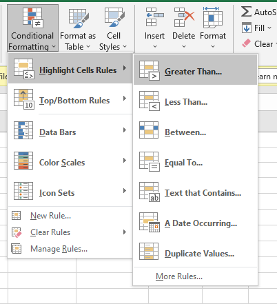
- A new window opens named Greater than asks you to enter a number.
- You must enter a number to highlight all selected cells greater than that number.
- Choose a highlight style that best suits you or you can set a custom highlight style and color by clicking Custom Format.

- Click OK to apply the formatting.
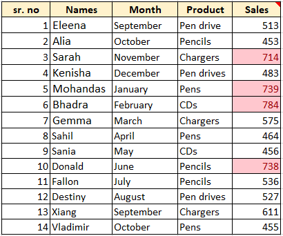
You can now find that all cells with values greater than 618.5 have been highlighted.
3. Highlighting cells with a value less than {value}
- Select the values in the database you want to apply conditional formatting to.
- Go to the Home tab.
- Under Styles, pull-down on Conditional Formatting.
- Hover over Highlight Cells Rules and select Less than.
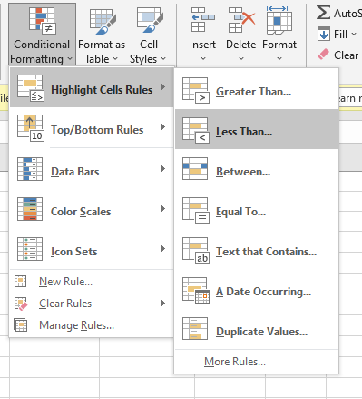
- A new window opens named Less than asks you to enter a number.
- You must enter a number to highlight all selected cells less than that number.
- Choose a highlight style that best suits you or you can set a custom highlight by clicking Custom Format.

- Click OK to apply the formatting.
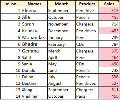
You can now find that all cells with values less than 618.5 have been highlighted.
4. Highlighting cells with values between two numbers
- Select the values in the database you want to apply conditional formatting to.
- Go to the Home tab.
- Under Styles, pull-down on Conditional Formatting.
- Hover over Highlight Cells Rules and select Between.
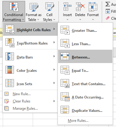
- A new window opens named Between asks you to enter two numbers.
- You must enter a minimum number and a maximum number to highlight all selected cells between those two numbers present in the database.
- Choose a highlight style that best suits you or you can set a custom highlight.

- Click OK to apply the formatting.
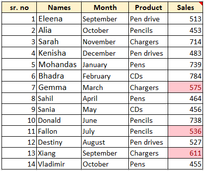
You can now find that all selected cells with values between 536 to 701 have been highlighted.
Also read: How to insert hyperlinks in Excel?
5. Highlighting cells with values equal to a number
- Select the values in the database you want to apply conditional formatting to.
- Go to the Home tab.
- Under Styles, pull-down on Conditional Formatting.
- Hover over Highlight Cells Rules and select Equal to.
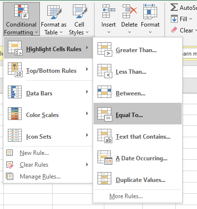
- A new window opens named Equal to asks you to enter a number.
- You must enter a number to highlight all selected cells equal to that number.
- Choose a highlight style that best suits you or click Custom Format to set a custom-colored highlight.

- Click OK to apply the formatting.
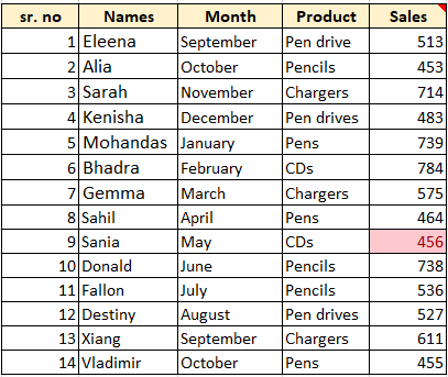
You can now find that the cell with the value equal to 456 has been highlighted.
6. Highlighting cells that contain a particular string
This conditional formatting rule can be applied only to textual data.
- Select the texts in the database you want to apply conditional formatting to.
- Go to the Home tab.
- Under Styles, pull-down on Conditional Formatting.
- Hover over Highlight Cells Rules and select Text that contains.
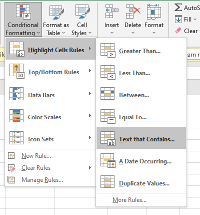
- A new window opens named Text That Contains to asks you to enter a text.
- You must enter the string to be highlighted across all selected cells containing in.
- Choose a highlight style that best suits you or click Custom Format to set a custom-colored highlight.

- Click OK to apply the formatting.
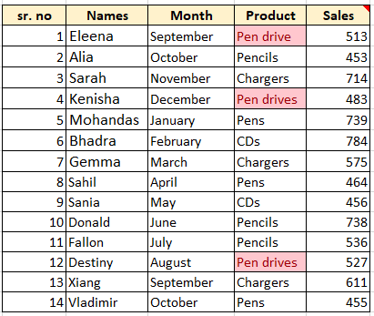
You can now find that all cells with the text containing “Pen drives” have been highlighted.
7. Highlighting cells with a particular date
This conditional formatting rule can be applied only to cells with dates.
- Select the dates in the database you want to apply conditional formatting to.
- Go to the Home tab.
- Under Styles, pull-down on Conditional Formatting.
- Hover over Highlight Cells Rules and select A Date Occurring.
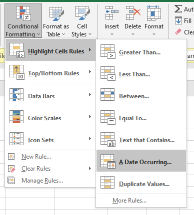
- A new window opens named A Date Occurring that asks you to choose a time in a month.
- You can select any day or times of the month to highlight all selected cells with that date.
- Choose a highlight style that best suits you or click Custom Format.
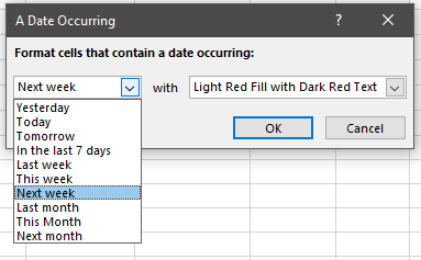
- Click OK to apply the formatting.
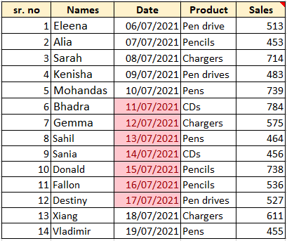
You can now find that the cells with the chosen dates or times of the month have been highlighted.
8. Highlighting cells with duplicate values
- Select the dates in the database you want to apply conditional formatting to.
- Go to the Home tab.
- Under Styles, pull-down on Conditional Formatting.
- Hover over Highlight Cells Rules and select Duplicate Values.
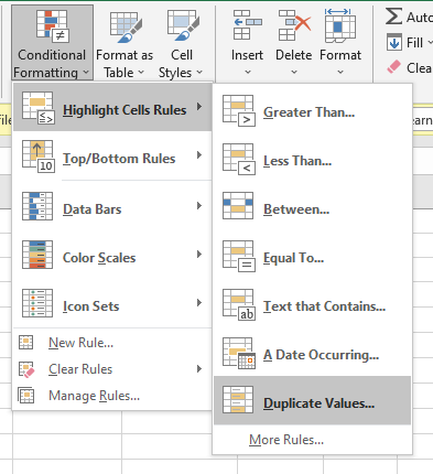
- A new window opens named Duplicate Values that asks you to either choose Duplicate or Unique.
- You can highlight cells with duplicate values via the first option and highlight all unique values except duplicate values with this formatting.
- Choose a highlight style that best suits you or click Custom Format for custom formatting color and style.
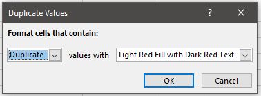
- Click OK to apply the formatting.
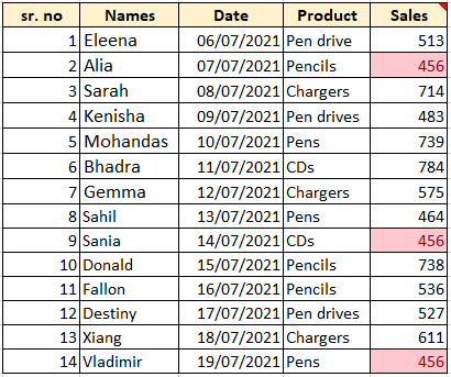
You can now find that all cells with duplicate values have been highlighted.
9. Highlighting Top or Bottom values
To highlight the top or bottom values in a database, follow these steps.
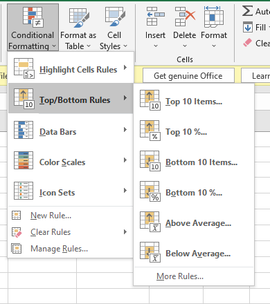
- Select the values in the database you want to apply conditional formatting to.
- Go to the Home tab.
- Under Styles, pull-down on Conditional Formatting.
- Hover on Top/Bottom Rules and select Top 10 items to highlight any number of top items you want in the database.
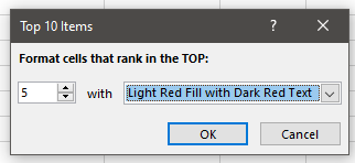
- Select the Top 10 items to highlight any number of bottom items you want in the database
- You can even choose to highlight the top or bottom cells based on a certain percentage by clicking Top 10 % or Bottom 10%.
- You can highlight all values with above or below average by clicking Below Average or Above Average.
- Click OK to apply the formatting.
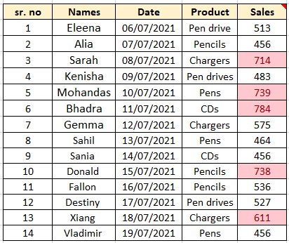
You can now find that all top 5 values in the database have been highlighted.
10 Applying custom fills to cells
- Select the values in the database you want to apply conditional formatting to.
- Go to the Home tab.
- Under Styles, pull-down on Conditional Formatting.
- Hover on Data Bars and select the desired gradient or solid color fill to apply to the values.
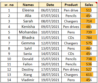
To apply colorful fills to every value in the database, here is what you can do.
- Select the values in the database you want to apply conditional formatting to.
- Go to the Home tab.
- Under Styles, pull-down on Conditional Formatting.
- Hover over Color Scales and select the desired color scales to be applied.
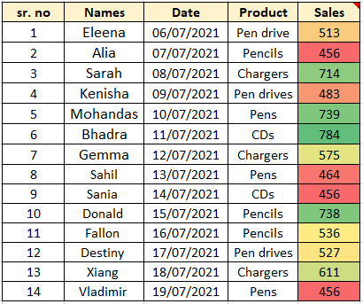
11. Applying custom icons to cells
- Select the values in the database you want to apply conditional formatting to.
- Go to the Home tab.
- Under Styles, pull-down on Conditional Formatting.
- Hover over Icon Sets and select any set of directional, shape, indicator, or rating icons for your datasets.
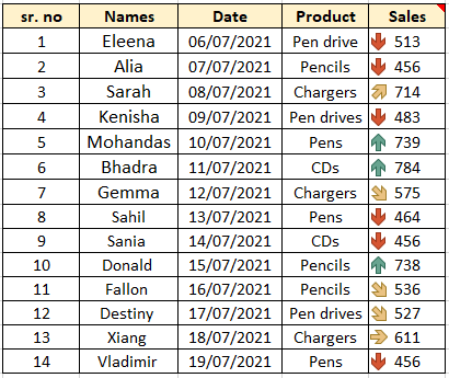
How to Remove Conditional Formatting in Excel?
Finally, after you have applied all these conditional formattings, there is definitely a way to remove them if you no longer need them or dislike them. Follow these steps to remove conditional formatting.
- Select the cells with applied conditional formatting.
- Go to the Home tab.
- Under Styles, pull-down on Conditional Formatting.
- Pull Clear Rules at the bottom.
- Select Clear Rules from Selected Cells.

You can find that rules and formats have been cleared from the selected cells.
Conclusion
This article was a detailed beginners’ guide to using conditional formatting in Excel. If you have any doubts regarding conditional formatting, feel free to comment below and we will respond with an answer to your questions!
