Are you interested in making searchable dropdown lists in Microsoft Excel? You’re at the right place! This tutorial is all about creating a searchable dropdown list in Excel.
If you’re on an older version than Office 365, and you want to make searchable dropdown lists without using the FILTER and UNIQUE functions in Excel, then this tutorial is made for you!
We will use a variety of simple formulas to make our dropdown list searchable. Searchable lists are convenient to handle and ease looking up values or terms in large databases.
Let’s get cracking!
Steps to create searchable dropdown lists in Excel
Let’s get started with this simple guide to creating a searchable dropdown in Excel. Here is the list of formulas we used to create the searchable dropdown list in this tutorial.
- SEARCH Formula
- ISNUMBER Formula
- IF Formula
- MAX Formula
- ROWS Formula
- VLOOKUP Formula
- IFERROR Formula
- OFFSET Formula
- COUNTIF Formula
To begin with, let us prepare a random name list that we will search in the dropdown list. Here’s a list of 30 random names.
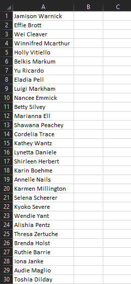
Now that the list is ready, we will start creating the searchable dropdown list. Follow the steps carefully.
First off, let’s choose a cell that will contain the dropdown list. You can give a custom cell color.
1. Use SEARCH() to find substrings
Now, let’s start with the technical part of the searchable list.
- Click on the adjacent cell to the first name in the list.
- Type the search formula in this cell.
- Type =SEARCH( and click on the cell with the dropdown list.
- Press F4 or Fn+F4 on your keyboard to lock the cell address.

- Put a comma and select the first name in the list.
- Hit ENTER.
You will see 1 displaying in that cell now.
- Double-click on the right side of that cell to auto-fill the formula in the entire column.
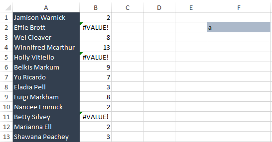
In this image above, we have searched for the term “a” in the search box that is displaying numbers in some cells and a VALUE error in some cells. The numbers denote the character position of “a” in these cells. Cells with the VALUE error indicate there is no character as “a” in that specific name.
2. Change SEARCH() output to TRUE or FALSE
The next step is to make these cells containing numbers display “TRUE” and cells without numbers as “FALSE” instead of the VALUE error. Follow the steps below.
- Click on the first cell with the SEARCH function.
- Edit the formula in the formula bar by adding the ISNUMBER formula before the SEARCH formula.
- In the formula bar, type ISNUMBER( after =
- Put a closing bracket at the end of the SEARCH formula.
- Hit ENTER.
- Autofill the new formula to the rest of the column.

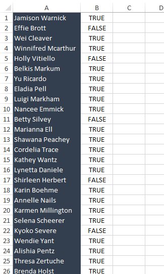
You can see cells with TRUE and FALSE values in them.
3. Convert TRUE values to incremental numbers
The next step is to display all TRUE values as incremental numbers. Here are the steps.
- Click on the first cell with the formula in it.
- In the formula bar, we will add the IF and MAX formulas to the existing formula.
- Type IF( after the bracket.
- Go to the end of the existing formula, and put a comma.
- Type MAX( and click on the cell above this cell. Insert a row if you do not have space above the cell.
- Put a colon (the cell address repeats)
- Press F4 or Fn+F4 to lock the first cell address.
- Close the bracket.
- Type +1 and put a comma, type 0).
- Hit ENTER.

- Autofill the formula to the entire column.
4. Test out the filter
Now, let us try searching for a term in the box and check if the incremental numbers are being displayed only for the searched term. For instance, we searched “ka” in the cell and hit ENTER.
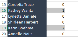
You can see that the two names starting with KA, that are, Kathey and Karin, have the numbers displayed as 1 and 2 respectively. So, this proves that we’re right on track.
5. Using ROWS() to lookup values
The next step is to use the ROWS function that will be used as the lookup value for the VLOOKUP function that we will use later in this tutorial.
- Click on the first adjacent cell to the cell with formulas.
- Type ROWS( and click on the first name in the list.
- Put a colon to let the cell address get repeated in the formula.
- Click on the first cell address of the two.
- Press F4 or Fn+F4 to lock the cell address.
- Close the brackets.

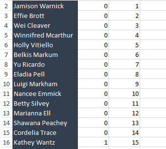
Now, double-click on the right side of the cell to auto-fill the formula in the entire column. You will see the row numbers being displayed in the column.
6. Add VLOOKUP to ROWS()
It’s time to add the VLOOKUP formula to the existing ROWS formula.
- Type VLOOKUP( after =
- Go to the end of the ROWS function and put a comma.
- Now, select the column ranges with the formulas and name list when asked for the table array.
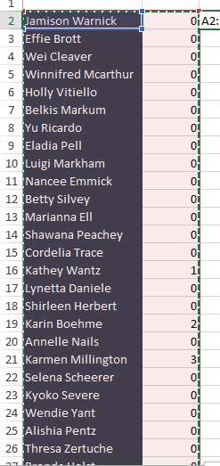
- Put a comma and type the number of the column that has the name list. Here, the names are listed in the 1st column, so, we wrote 1.
- Put a comma and type 0 for the exact match.
- Hit ENTER.
You can see all names in this column now after auto-filling the range data.
Note that we have shifted the column with the SEARCH and other formulas to the left of the name list column. You can follow the same in case you’re having troubles with the VLOOKUP function.
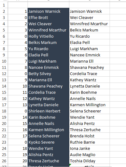
We will search for the “Ka” again to check if the function is working correctly.
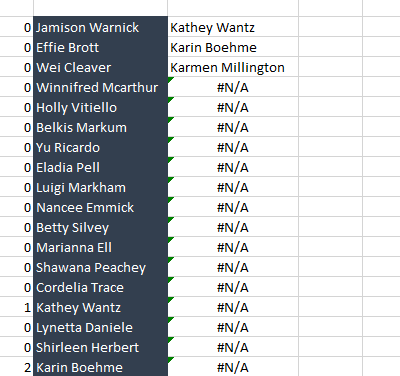
You can see that names with “Ka” in them are being displayed in the first three cells. The rest of the cells are displaying the N/A error.
Let’s fix this problem now.
9. Hide #N/A output
Here are the steps to hide the N/A error message in the empty cells.
- Edit the cell with the VLOOKUP formula again and add the IFERROR formula to it.
- Type IFERROR( after =
- Go to the end of the formula and put a comma.
- Type “”)
- Hit ENTER.
- Autofill the formula to the entire column.

The double quotes denote “Blank” in Excel. Now, Excel will leave the cells blank if there is any error shown in empty cells.
The further steps are about using the OFFSET and COUNTIF functions and displaying search terms in a dropdown list. It brings us to the end of the first part of this tutorial.
Conclusion
This tutorial was Part 1 guide to creating a searchable dropdown list in Microsoft Excel. Part 2 is all about using more crucial formulas to make the searchable list fully functional. Stay tuned for more FREE prime automation tutorials on QuickExcel!
