We solve and deduce complex problems by analysing data using the formula in MS Excel, but these formulae are not foolproof and anyone with the privilege to access the sheet can fiddle with each & every formula to the extent that it becomes a web of spaghetti!
It would really cost us precious time when the formula created has been tampered and we need to get down to the roots of it for troubleshooting the same. In this article, we are about to venture into a technique that would restrict those evildoers’ mischief. How are we going to do it, you ask?
Locking the Cells!
Locking Cells with Formula
Have a look at the below dataset.

Everything seems to be alright at the first look, but pay a bit of attention to the details & you would be getting it – columns G & H are filled with formulae.

The above view can be made possible when one uses the keyboard shortcut, CTRL + ` (tilde). To prevent any mishaps from happening, we would be needing to protect these formulae & we would do just that. But, we would be needing to do some pre-requisites before we get on with the protection.
Hit CTRL+A to select the entire sheet and click on the following to open the Font Settings, as shown in the below image.
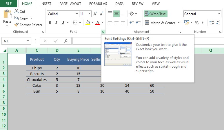
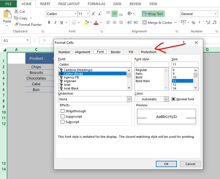
One might also use the keyboard shortcut as given in the above image for opening the Font Settings. A dialog box appears as shown below. Select the Protection tab within that, as indicated.
Once done, one can view a checkbox Locked being ticked as shown below.
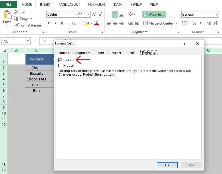
Remove the tick off the checkbox & click OK.
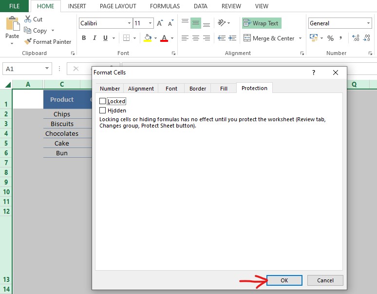
This follows by selecting the cells containing the formula alone, as shown below.

Now, one shall go through the process of opening the font settings again. The Protection tab is selected, but this time, we are going to tick the Locked Checkbox as shown in the below image & click OK.
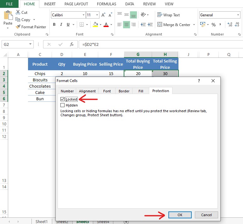
What we have done now is to change the default mode of MS Excel to protect the entire sheet & restrict it to protecting the cells which we have selected.
It’s time, we end this task by navigating our way to the Review tab as shown in the below image.
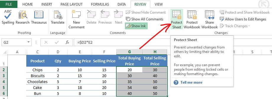
Once you’re in the Review tab, look out for the Protect Sheet option. It would be in the position as indicated in the above image. Click on that option & a pop-up would find its way to the screen.
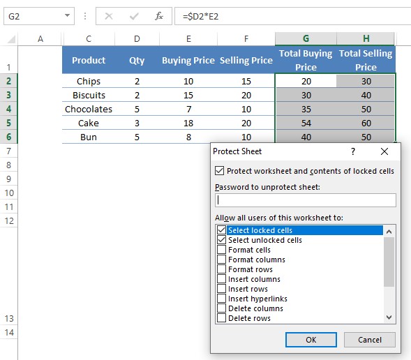
This pop-up would have within it a list of options to choose from, but for our case, the options checked by default would serve the purpose. Type a password which is easy to remember, since if this has been forgotten, there’s no ‘Forgot Password’ in MS Excel & the file would remain a mystery. Click OK once the password is typed.
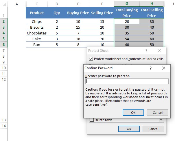
Once, OK is clicked the above pop-up appears asking to re-enter the password. One can understand the gravity of the situation with the password if the all-flexible Excel prompts its user to confirm it.
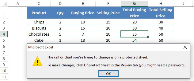
Click OK again & all the selected formulae get protected! Even if someone tries to edit it, the following message would appear.
Conclusion
We have reached the end of this article. Do have a look at this article, to know how to draw a line in MS Excel. Nevertheless, QuickExcel has numerous other articles, which would be of great help to you when it comes to understanding the nuances of working with MS Excel. Cheers!
