Don’t compare apples with oranges!
A common saying that we all would have come across at least once. When one tends to carry out a comparison, one ought to make sure that both the entities that are being compared are placed on a level playing field. The same logic also holds good when it comes to MS Excel.
Also read: How to calculate Z-Score in Excel?
When comparing a list of data, for instance, the scores of the pupil in a class for a subject upon 100 marks & another subject upon 200 marks, won’t it be better if one can adopt a universal scale within which any value can be transformed & fitted in.
By this, both the scores, out of 100 & 200 are reduced down to a common scale such that we can compare the performance of the pupil with ease. This technique is called Normalization of data & in this article we are going to get into its greater depths, analysing the formula involved & how to put it into use.

Given above is a list of marks obtained by 5 students. It can be seen the scale on which these marks are awarded varies. So, let us see how to normalise them.
This makes us go for a search into the arsenal of MS Excel to find the formula in-built to serve the very purpose – STANDARDIZE!
The following is its syntax showing the prerequisites for the formula to function,
=STANDARDIZE( x, mean, standard_deviation)
While the other 2 entities are self-explanatory, ‘x’ here denotes the individual entity which in this case would be the score of each student.
Finding the Mean:
The first step is to find the arithmetic mean for each of these score lists using the formula,
=AVERAGE(number_1, number_2, ….)
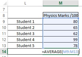
At the bottom of the Physics marks column, one shall construct this formula by selecting cells with the scores as depicted in the below image.

The same is also to be done for the History score list too & we get the mean for both the score list as given below.

Finding the Standard Deviation:
The Standard Deviation can also be calculated by an in-built Excel formula whose syntax is given below.
=STDEV.S(number_1, number_2, ….)
STDEV.S takes into account only numerical values & ignores all textual and logical values. It is also chosen since the 5 students are a sample of the entire class strength. The Formula is constructed for both score lists as shown below.

Hit ENTER & the results shall be displayed.

Using STANDARDIZE:
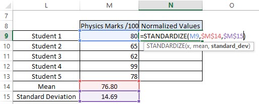
A column is created to the right of the Physics score list to determine all the normalised values using the STANDARDIZE formula as shown below.

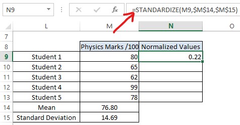
Hit enter & the normalised value calculated shall be displayed as shown below.

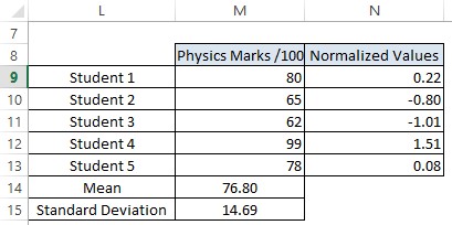
It could be noted that the cells M14 & M15 have been referred within the formula by a dollar sign ($) preceding the alphabet & number. This is to fix those cell references when the formula is being copied to the other cells below. Once the formula is copied the results would be similar to those in the below image.

Similarly, the normalised values for History scores can also be calculated by constructing the same formula referencing to the respective Mean & Standard Deviation as shown below.

Now all the scores have been reduced to the same scale (0’s, +1’s & -1’s), it would now be easier to compare the student’s performance in both categories within a similar range.

Summary
Now that we have reached the end of this article, here’s something that elaborates on How to Calculate Days in MS Excel? There are also numerous other articles in QuickExcel that can help you better understand MS Excel. Cheers!
