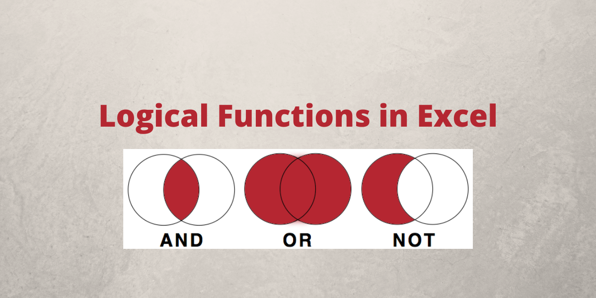
Logical functions in Excel help make comparisons and arrive at a logical conclusion. Here are the logical functions available in Excel and how to use them with examples.
List of Logical Functions
Let’s go over the list of logical functions that are available in excel and learn how we can use them in our day-to-day work.
1. AND function
AND function is one of the logical functions in Excel, which determines whether all criteria in a test are TRUE. it returns TRUE if all of its parameters are TRUE, and FALSE if one or more arguments are FALSE.
Syntax: AND(logical1, [logical2], …), where logical1 is the first condition you want to test is one that can be TRUE or FALSE and logical2… are optional and additional conditions up to a maximum of 255 conditions.
The following example shows the use of AND function:
- Select the cell where you want to display the result.
- Type =AND(A1>50,B1<50) where cells A1 and B1 contain numeric values.

- Press the Enter key to display the result.

2. FALSE function
The FALSE function in Excel returns the logical FALSE value.
Syntax: FALSE(), it has no arguments. Microsoft Excel will read the word FALSE without parentheses as the logical value FALSE if you write it directly onto the worksheet or into a formula.
3. IF function
One of Excel’s most used tools is the IF function, which allows you to create logical comparisons. An IF statement can have two possible outcomes. If the comparison is TRUE, the first result is returned; if the comparison is FALSE, the second result is returned.
Syntax: IF(logical_test,value_if_true,[value_if_false]), where logical_test is the comparison you want to test, value_if_true is the value to be returned if the logical_test is TRUE, and value_if_false is the value to b returned if the logical_test is FALSE. The following example shows the use of the IF function:
- Select the cell where you want to display the result.
- Type =IF(A1>B1,”A1>B1″,”A1<B1″) where cells A1 and B1 contain numeric values.

- Press the Enter key to display the result.

4. IFERROR function
The IFERROR function can be used to catch and manage errors in a formula. If a formula evaluates to an error, IFERROR returns a value you specify; otherwise, it returns the formula’s result.
Syntax: IFERROR(value, value_if_error), where value is the condition to be checked for #N/A, #VALUE!, #REF!, #DIV/0!, #NUM!, #NAME?, or #NULL! error and value_error is the custom message to be returned if the formula evaluates to an error. The following example shows the use of the IFERROR function:
- Select the cell where you wan to display the result.
- Type =IFERROR(A2/B2,”Error in calculation”) where cells A2 and B2 contain the dividend and divisor respectively.

- Press the Enter key to display the result. As, you can see the divisor is zero, so a #DIV/0! should be returned. IFERROR fucntion catches the error and returns the custom message.

5. IFS function
The IFS function determines whether one or more criteria are met and returns the value corresponding to the first TRUE condition. With several criteria, IFS can replace nested IF statements and is considerably easier to read.
Syntax: IFS(logical_test1, value_if_true1, [logical_test2, value_if_true2], [logical_test3, value_if_true3],…), where logical_test1 is the first comparison you want to test, value_if_true 1 is the value to be returned if the logical_test1 is TRUE and the same follows for other conditions. The following example shows the use of IFS function:
- Select the cell where you want to display the result.
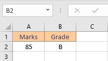
- Type =IFS(A2>89,”A”,A2>79,”B”,A2>69,”C”,A2>59,”D”,A2<=59,”F”) to assign letter grades on the basis of marks obtained.

- Press the Enter key to display the result. The value returned is “B” as 85>79 and 85<90.
6. NOT function
The NOT function returns the inverse of its argument’s value. It is frequently used to extend the utility of other functions that perform logical tests.
Syntax: NOT(logical), where logical is a value or expression that may be tested to determine whether it is TRUE or FALSE. The following example shows the use of the NOT function:
- Select the cell where you want to display the result.
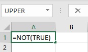
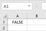
- Type =NOT(TRUE), to reverse TRUE value to FALSE.
- Press the Enter key to display the result.
7. OR function
The OR function returns TRUE if any of its parameters are TRUE and FALSE if all of its arguments are FALSE.
Syntax: OR(logical1, [logical2], …), where logical1, logical2, logical3 etc, are conditions to be evaluated for TRUE and FALSE values. The following example shows the use of the OR function:
- Select the cell where you want to display the result.
- Type =OR(A1<50,B1>50) where cells A1 and B1 contain numeric values.

- Press the Enter key to display the result.

8. SWITCH function
The SWITCH function compares one value called the expression to a list of values and returns the first matched value as the result. If no match is found, a default value is returned.
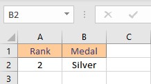
Syntax: SWITCH(expression, value1, result1, [default or value2, result2],…[default or value3, results]), where expression is the value to be compared, value1… are the values to compare an expression to, and result1… are the results to be returned corresponding to the matching value of the expression. The following example shows the use of the SWITCH function:
- Select the cell where you want to display the result.
- Type =SWITCH(A2,1,”Gold”,2,”Silver”,3,”Bronze”) to decide medals on the basis of rank in cell A2.

- Press the Enter key to display the result.
9. TRUE function
The TRUE function in Excel returns the logical TRUE value.
Syntax: TRUE(), it has no arguments. Microsoft Excel will read the word TRUE without parentheses as the logical value TRUE if you write it directly onto the worksheet or into a formula.
10. XOR function
The XOR function returns a TRUE value when the number of true inputs is odd otherwise it returns FALSE. Syntax: XOR(logical1, [logical2],…), where logical1, logical2, logical3 etc, are conditions to be evaluated for TRUE or FALSE values. The following example shows the use of XOR function:
- Select the cell where you want to display the result.
- Type =XOR(A1>50,B1<50,C1<25) where cells A1, B1 and C1 contain numeric values.

- Press the Enter key to display the result. The XOR fucntion returns FALSE value as 2 conditions are TRUE and 2 is an even number.

Conclusion
In this article, we learned about the various logical functions in Excel.
