Collaboration is a vital approach to sustain & boost the performance of a team. What else shall be put into practice rather than sharing information through spreadsheets? Though these sheets may be quite quaint, they have indeed lasted the tests of time & continue to stay for a reason – their flexibility. But this very flexibility might cause trouble in some instances!
With too many people accessing a file, it is of grave importance to safeguard the data that has previously been recorded. At times, some data are never to be changed since they would be directly linked with other data visualisation tools.
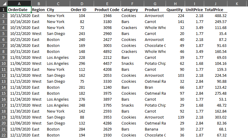
In this article, we shall elaborate on the sequence of steps to lock the columns & we shall be using the below tabulation to demonstrate that.
Locking Columns in MS Excel:
One shall get started by selecting all the contents of the sheet by pressing CTRL+A and then opening the Font settings option by clicking on the button as shown in the below image.
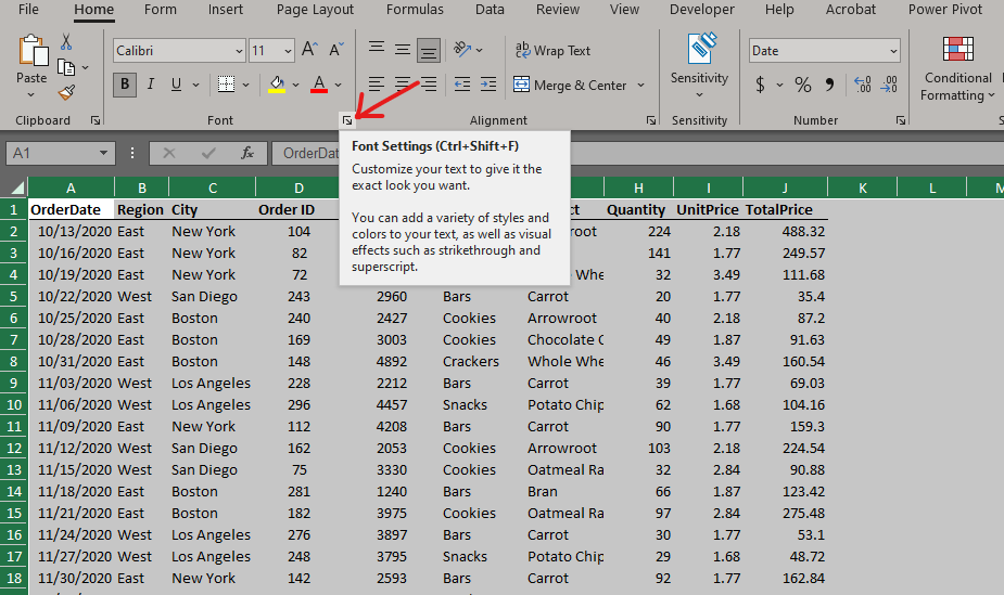
For the people inclined toward keyboard shortcuts, they would be better off with CTRL+SHIFT+F to open the Font Settings. Much caution is to be exercised while executing this shortcut, as the keys ought to be pressed one after the other & not simultaneously. Doing the latter would only render the shortcut unfeasible. Once done, the Format Cell dialog box appears as shown below.
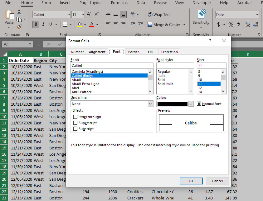
Choose the Protection Tab, in the above dialog box to uncheck the Locked checkbox. Then, click OK.
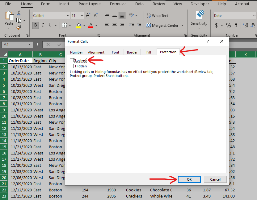
The dialog box is now closed & the vast sheet with all its details is now left for us to look at.
The next step is to select those columns which are needed to be locked. In this case, we would be trying to lock the contents of the columns titled Order ID & Product Code, under the pretence that they are key entities which are not supposed to be altered by any visitor to the file.
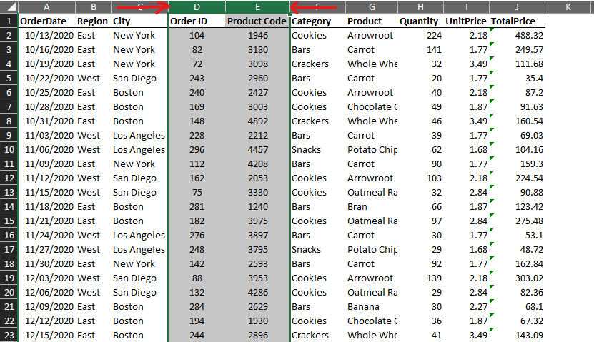
Now, one shall repeat the same steps as done previously by opening again the Format Cells dialog box, going again to the Protection tab, but this time, ticking the Locked checkbox!
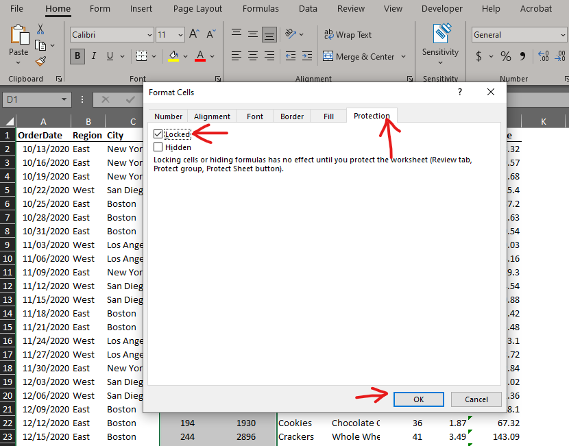
So far, we have covered the steps needed to convey MS Excel which cells to protect when the sheet gets protected. Now, we shall move on to the part where we protect the sheet. This is relatively simple, needing us to navigate our way to the Review tab & locate the Protect Sheet option as shown in the below image.
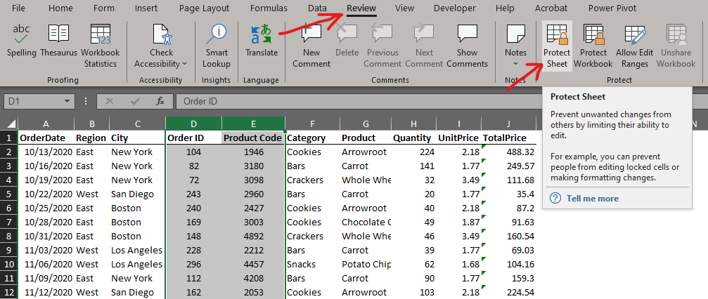
One shall now click on the Protect Sheet option, only to look at a dialog box prompting to enter a password.
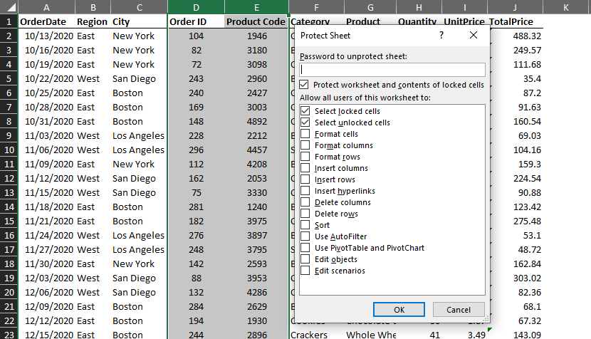
A password of your choice can be typed in here & once OK is hit; another dialog box appears prompting to confirm the password. One needs to bear in mind that if the password given once forgotten, shall never be retrieved since MS Office has not blessed us with that feature yet!
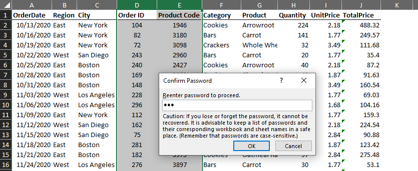
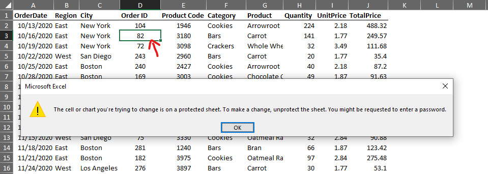
Click OK & try editing the contents of any cell in the selected columns. An alert as shown below shall appear.
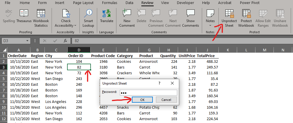
One can always unlock the contents by navigating again to the Review tab & select Unprotect Sheet! A dialog box shall appear seeking a password. Upon entering the right password & hitting OK, the locked columns become editable.
Conclusion:
Now we have reached the end of this article detailing how to lock columns in MS Excel & hope that got what you were looking for. But what if you want to know more about the operations that can be done with the columns in MS Excel? How to Move a Column in MS Excel? elaborates on the necessary details. QuickExcel has numerous other articles too that can come in handy for those who are in a quest to know something more in MS Excel. Cheers!
