Filters or hiding cells serve the purpose when the underlying information belongs to the same category. But for those which have subsets, as in small groups within each larger group, these features provided by MS Excel does not deem to be fit. What else does Excel’s bags of tricks have got to offer on this occasion?
Also read: How to Hide Cells in MS Excel?
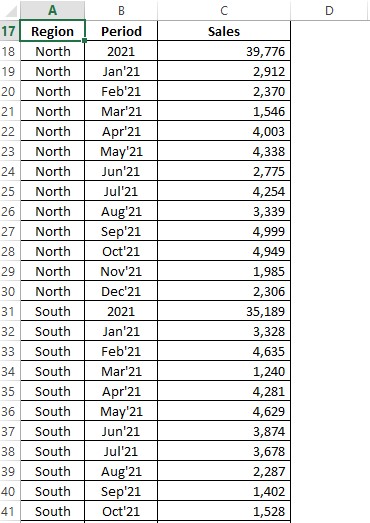
We are going to have a look at just that in the following sections & we would be using the following tabulation to demonstrate through each of the below methods,
- Selecting from Data Tab
- Keyboard Shortcut
Grouping of Rows:
To group any given data, one has to look into the commonalities that exist, which in the above dataset is the time period for 2021, which has been summarised under each Region. The given tabulation consists of four different regions with the sales details for a period of 12 months listed under each region.
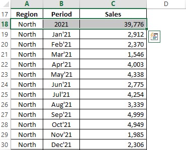
There also exists a summary which contains the total of the sales numbers for that year at the very beginning.
That’s all for the briefing & your mission, should you choose to accept it is to group all 12 months under each region such that it would be easier to compare any two regions against each other in a single click.
Method 1 – Selecting from Data Tab:
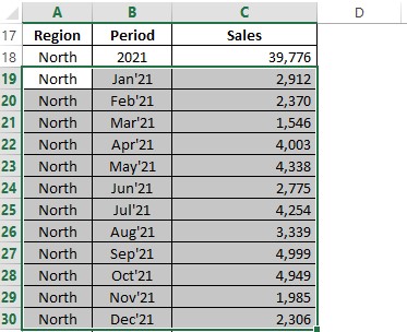
Let us get started by selecting the rows of the 12 months given under the North region as shown in the below image.

Navigate your way using the cursor to the Data tab & that is where you will be finding the Group option.
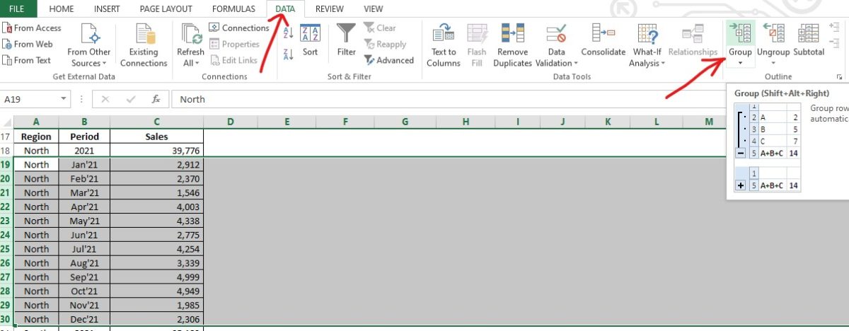
What are you waiting for? Click on that option!
The following changes would be visible on your screen in a jiffy.

“Yeah, yeah! Enough of gimmicks & can you tell me what to do with those buttons in the above image?”
I’ve foreseen these voices of yours & here is what one can do. Click on the minus (-) button to collapse all the 12 months under the North region. Once done, the minus (-) button transforms itself into a plus (+) button & the 12 months has gone with the wind.
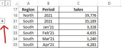
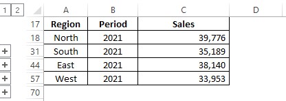
Repeat the same procedure for the other regions too such that all the rows with the months from Jan to Dec get hidden only to be summoned by the click of the plus (+) button.
Method 2 – Keyboard Shortcut:
The part where we select the rows of the months under a region remains the same as stated in the previous method. The difference kicks in now.
Rather than moving the cursor, one shall place the fingers over the keys of the keyboard. Which keys do you ask?
These!
SHIFT + ALT + RIGHT ARROW KEY (→)
Much emphasis is on pressing the keys one after the other, similar to the way CTRL+C or CTRL+V is exercised. Trying to pull off anything else, would only render the execution of this shortcut unfeasible.
After the above keys are pressed in the same sequence, the selected rows would be collapsed as shown below.

The same technique is repeated to group & collapse the months of the other regions too.

Conclusion:
Hope the article was informative. Here is an additional lead to an article that might interest you! To know how to freeze columns in MS Excel, do have a look at this article. QuickExcel has numerous other articles too which could help you with that one thing that you’re trying to do with MS Excel right now. Cheers!
