6 Simple Ways to Format Cells in Excel in Less Than 5 Minutes

This article is a detailed tutorial on how you can format cells in Excel. We will learn to adjust cell sizes, lock and unlock cells, protect sheets, and much more with the help of the Format tool in Excel.

Steps to format cells in Excel

The Format tool is situated in the Home tab in the Cells section in Excel. There are multiple uses of this tool like adjust cell sizes, locking unlocking them, or hiding or unhiding rows and columns, etc. We will learn each feature one by one to learn in detail about this tool in Excel.

Adjusting cell sizes in Excel

Let’s begin by understanding how to adjust the cell sizes in Excel.

1. Adjusting row height

The easiest way to adjust the row height is as follows.

• Rest the cursor on the line between two rows. Your cursor should change to a black plus icon with an arrow at its top and bottom.
• Left-click and move the line up or down to increase or decrease the height.

Another way to adjust the row height is by using the Format option in Excel.

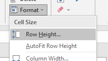
The first option in the Format cells tool is Row Height.

• Remain in the row for which you want to adjust the height.
• Go to the Home tab.
• Click on Format under the Cells group
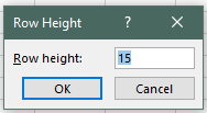
• Select Row Height. The default height of a row is 15 but you can adjust it as per your liking.

• A window named Row Height opens displaying the current height of the row.
• Click OK when you’re done.

To autofit row height, follow these steps.

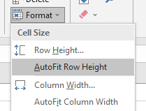
• Click on a cell in the row for which you want to adjust the height.
• Select the AutoFit Row Height option in the Format tool.

The row is automatically adjusted to the default height.

2. Adjusting column width

The easiest way to adjust the column width is as follows.

• Place the cursor on the dividing line between two columns. Your cursor should change to a black plus icon with an arrow at its right and left.
• Left-click and move the line to the right or left to increase or decrease the column width.

Another way to adjust the column width is by using the Format option in Excel.

• Click on a cell in the column for which you want to adjust the width.
• Go to the Home tab.
• Click on Format under the Cells group
• Select Column Width. The default width is 8.43 but you can adjust it as per your liking. You can check for the standard width by clicking on the Default Width option in the tool.

• A window named Column Width opens displaying the current width of the column.
• Click OK when you’re done.

To autofit column width, follow these steps.

• Click on a cell in the column for which you want to adjust the width.
• Select the AutoFit Column Width option in the Format tool.

The column is automatically adjusted to the default width.

Steps to hide/unhide rows, columns, or sheets in Excel

Now, let’s learn to hide or unhide rows and columns and even sheets in Excel.

Also read: How to Hide and Unhide Columns in Excel?

1. Hide or unhide rows

To hide or unhide rows, follow these steps.

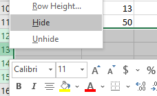
• Right-click on the row you want to hide.
• Or, select multiple rows you want to hide.
• Right-click on row and select Hide.

You can see that all rows between 11 and 16 have been hidden.

To unhide hidden rows, do as follows.

• Select the rows between which there are hidden rows.
• Right-click and select Unhide.
• Or simply double-click on the line between two rows where there are hidden rows until your cursor turns into a black plus with two parallel lines in the middle.

All hidden rows will now be seen. Another way to hide or unhide rows is by using the Format tool in the home tab.

• Select the rows you want to hide.
• Go to the Home tab.
• Click on Format under the Cells group
• Click Hide & Unhide under Visibility.
• Click Hide Rows.

To unhide hidden rows, do as follows.

• Select the rows you want to unhide.
• Go to the Home tab.
• Click on Format under the Cells group
• Click Hide & Unhide under Visibility.
• Click Unhide Rows.

Steps to organize sheets in Excel

Let’s learn to rename, give a color, protect, move, or copy a sheet in Excel with the help of the Format tool.

To rename a sheet, do as follows.

• Double-click the sheet name.
• Enter a custom name you like.
• Press ENTER.

Another way to rename a sheet is using the Format options.

• Remain in the sheet for which you want to change the name.
• Go to the Home tab.
• Click on Format under the Cells group
• Click on Rename Sheet.
• Type a custom name you like.
• Press ENTER.

To apply a tab color to the sheet, do as follows.

• Remain in the sheet to which you want to apply color to.  
• Go to the Home tab.
• Click on Format under the Cells group.
• Pull Tab Color.
• Select a color you like for your sheet tab.

You can see that the first sheet’s tab has been colored green.

To move or copy a sheet in Excel, follow these steps.

A sheet can be moved within a workbook or from one workbook to another.

• Hold and drag the sheet you want to move within a workbook or to a different workbook.
• Or, go to the Home tab.
• Click on Format under the Cells group.
• Click on Move or Copy under Organize Sheets.

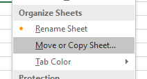
• A window named Move or Copy opens.
• Select (move to end) at the bottom to move the sheet at the last.
• Or select another sheet’s name before which you the current sheet to be placed.
• Click OK when you’re done.
• If you only want to create a copy check Create a Copy below and hit OK.

Recommended Read: How to Delete a Sheet in Excel?

To password protect a sheet in Excel, follow these steps.

• Stay in the sheet you want to protect.
• Go to the Home tab.
• Click on Format under the Cells group
• Click Protect Sheet under Protection.

• A window named Protect Sheet opens.
• Select the contents you wish to protect in the sheet.
• Set a password if you like in the top dialogue box.

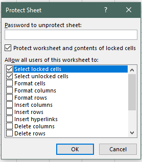
• Click OK.

Your sheet is now protected from other users with a password. This will disable other users from making changes to a sheet that is password protected.

Learn more here: How to Password Protect in Excel?

To unprotect a sheet.

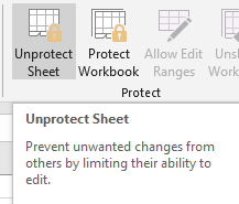
• Go to the Review tab.
• Click Unprotect Sheet.
• Enter the password (if any).
• Click OK.

Steps to lock cells in Excel

The cell locking feature becomes useful when you protect your worksheet and you only want certain cells in the sheet to be manipulated by other users and the rest of the cells to be locked.

First, we will lock the entire sheet and then we unlock the cells we want to allow manipulation. Here are the steps.

Our goal is to unlock the white cells and lock the contents in the orange cells.

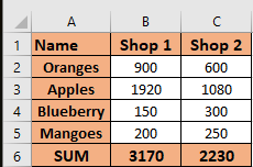
• Select the entire sheet by pressing CTRL+A on your keyboard or click on the grey arrow icon on the top left corner of the sheet.

• Right-click on the selection.
• Click on Format Cells.
• Go to the Protection tab.
• Check Locked.
• Click OK.

Now we must unlock the cells that we want to be manipulated.

• Select the cells you want to keep unlocked
• Right-click and select Format Cells.
• Uncheck Locked in the Protection tab.
• Click OK.

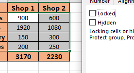
Now protect the sheet and check if it allows manipulation in locked cells.

• Go to the Home tab.
• Click on Format under the Cells group
• Click Protect Sheet under Protection.
• Set a password if you like in the top dialogue box.
• Click OK.
• Try typing in a locked cell. It should show this message.

Conclusion

This was all about the format tool in Excel. If you have any doubts regarding the format tool in Excel, email us and we will get back with help!

Reference: EasyClick Academy