How to Freeze Panes, Split a Sheet, and Hide Windows in Excel

This tutorial is a detailed guide to freezing rows and columns in Microsoft Excel. We will learn to freeze panes, split a sheet, and hide windows in Excel with the help of significant examples and supporting images.

Also read: 6 Simple Ways to Format Cells in Excel in Less Than 5 Minutes

Steps to Freeze Panes in Excel

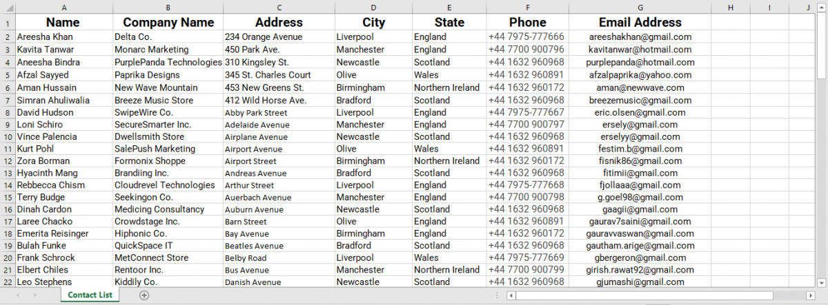
Let us get started by taking an example of a database of client contact details.

Steps to freeze the top row

To freeze the top row, follow these steps.

Go to the View tab.
Click Freeze Panes.
Select the second option named Freeze Top Row.

You can see that the top row in the sheet is frozen while scrolling.

To unfreeze the top row back to normal, do as follows.

Go to the View tab.
Click Freeze Panes.
Select Unfreeze Panes.

The top row is unfrozen now.

Steps to freeze the first column

To freeze the first column, follow these steps.

Go to the View tab.
Click Freeze Panes.
Select Freeze First Column.

You can see that the first column is frozen successfully.

Steps to freeze columns and rows at the same time

To freeze both the first column and the top row at the same time, do as follows.

Select a cell that is below the top row and adjacent to the first column.
Go to the View tab.
Click Freeze Panes.
Select Freeze Panes.

You can see that the top row and the first column together are frozen.

Steps to freeze multiple columns

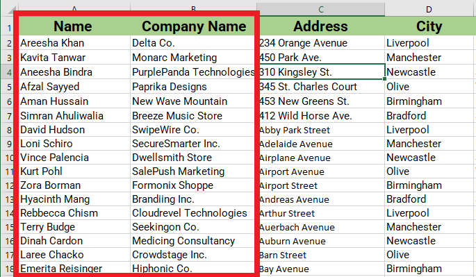
To freeze multiple columns excluding rows, do as follows.

Click on a cell in the top row.
Select the next column to the right to the multiple columns you want to be frozen. For example, if you wish to freeze the first two columns, select the 3^rd column.
To select an entire column press, CTRL+SPACE on your keyboard.
Click Freeze Panes in the Freeze Panes option.

Both columns are frozen now.

Click Unfreeze Panes to unfreeze the two columns.

Steps to freeze multiple rows

To freeze the multiple rows excluding columns, do as follows.

Click on a cell in the first column and the row below the multiple rows you want to freeze. For example, select the 4^th row if you wish to freeze the top 3 rows.
Click Freeze Panes in the Freeze Panes option.

Your rows are frozen successfully.

Steps to split rows and columns in Excel

Let us learn to use the Split tool in Microsoft Excel. The Split tool is in the View tab in the Window group in Excel.

This tool divides a sheet into four sections to compare a part of the database with its other part.

The split tool functions in the same manner as the Freeze Panes tool in Excel.

Meaning, if you have selected a cell in the 4^th column and 11^th row, then the Split tool will split the sheet between the 3rd and 4^th column and 10^th and 11^th row.

Let us depict this with an example.

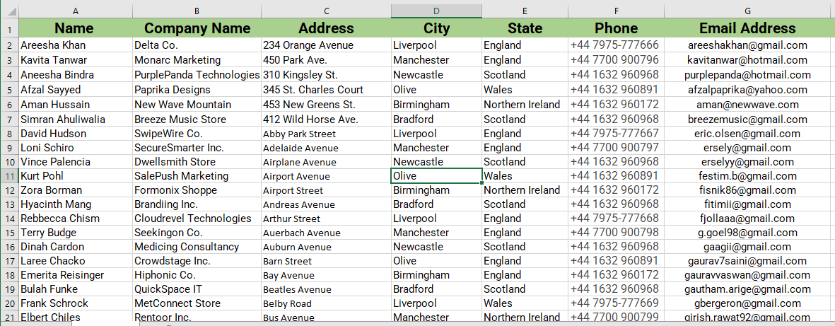
In this example above, we selected a cell with an entry named Olive located in the 4^th column and 11^th row.

Go to the View tab.
Click on Split.

You will see that the sheet divides into four parts with a grey line.

You can scroll each division separately to compare the data in a single database with ease.

Steps to manage multiple windows in Excel

Before we begin to hide a window in Excel, we must first learn to open a new window of the same file on your system. In the View tab, there is an option called New Window.

Choosing this option will open an identical Excel file in a new window. You will have all the sheets you created in the previous window opened in the new window in the same manner as in the image below.

Arranging windows side-by-side

To arrange the two windows appropriately, do as follows.

Go to the View tab from a random window.
Click on Arrange All.
Choose an option from the new window that opens. These options will arrange the two windows according to the arrangement you choose.
We have selected the vertical arrangement for a better view.

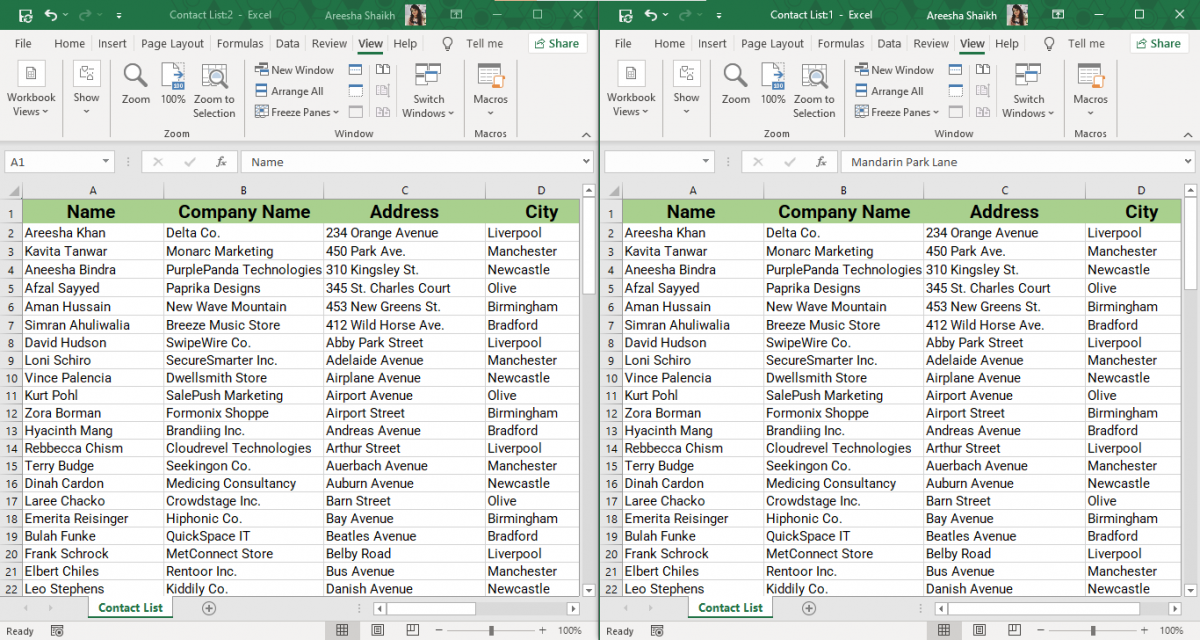
Or you can simply choose the View Side by Side option in the View tab to get the vertical arrangement for all windows at once.

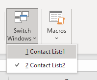
If there are more than two windows and you’re finding it difficult to switch between windows, then here’s what you can do.

In the View tab, pull down on the Switch Windows option.
Select the window number you want to switch.

Steps to hide windows in Excel

To hide a window, do as follows.

Open the window you want to hide.
Go to the View tab.
Click Hide.

The window is hidden but not closed.

To unhide a window back again, follow these steps.

Go to the View tab from a random window.
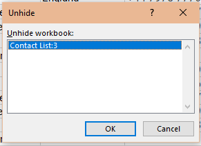
Click Unhide in the Window group.
A window opens, showing all your hidden windows.
Select the window you want to unhide.
Click OK.

Conclusion

This tutorial was about hiding and unhiding windows, splitting sheets into different parts, and freezing and unfreezing rows and columns in Microsoft Excel.

Reference: Microsoft