How dare they? Sneaking in whenever they want & waiting just for the moment where they can ruin everything – those stealthy duplicates. For reasons various, these guys could be found in any datasheets without any exceptions, unless there is some foolproof mechanism in place to prevent them from doing so.
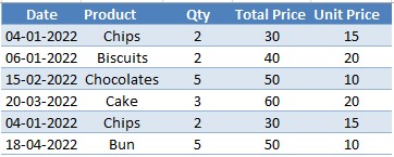
In this article, we shall look into the methodology to identify these duplicates and go even better – counting how many of them are present! We’d be using the following dataset to count the duplicate values present under the Date column.
Filtered Sub-Totalling
In this technique, one would be combining two different commands & utilising them to know the count of cells in the entire column. First, let us set the stage for counting the entire column & then get on with counting the duplicates in specific.
We get things moving by applying a Filter to the header row, which in this case is row 1. Select all the contents of row 1 as shown in the below image.

Once done, select the Filter option within the Home tab by clicking on the Sort & Filter group as shown in the below image.

For those who are fond of keyboard shortcuts, the same can be done by pressing CTRL, SHIFT & L keys one after the other. Exercise care while doing this since the requirement here is to press the keys one after the other & not simultaneously.
CTRL + SHIFT + L
Also, it is to be noted that the finger pressing the CTRL key should continue to press it, while the SHIFT key is being pressed & both the CTRL and SHIFT keys will be continued to be pressed while the letter key ‘L’ is hit.
Carrying out either of the above-mentioned ways would result in the filters getting applied to the headers as shown in the below image.

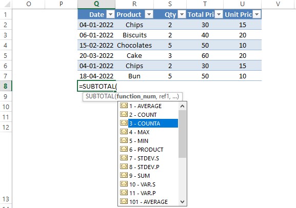
Now, it’s time that we include SUBTOTAL to count the total number of cells under column Q. One can always search within the Formulas Tab to select this formula. But before that, click on the cell below the last entry of Column Q to make it the active cell.

Then, we type SUBTOTAL with an EQUALS (=) sign at the beginning within cell Q8. Once done, the following list of options would appear and since our intent is to count the non-empty cells, we choose 3 – COUNTA.
Then, the entire cells in the column are chosen as shown in the below image.
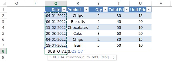
Include the closing bracket & hit ENTER to get the total count of entries in the selected range displayed within the cell.

Highlighting Duplicates:
It all comes down to using the filter option on the Date and selecting a particular colour to narrow down only to the duplicates. Which colour do you ask?
Enter HIGHLIGHT DUPLICATE VALUES!
This is one of the various options available in the Conditional Formatting menu. Select all the entries under the Date column & choose the option as shown in the below image.
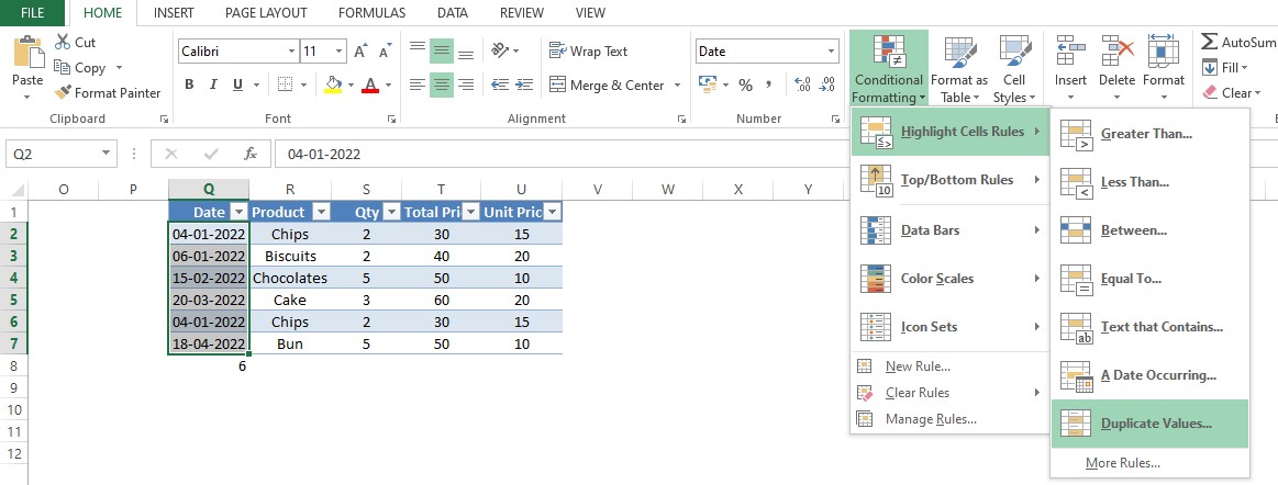
After the choice is made, there would be a prompt seeking to validate the colour needed to highlight the duplicates. In this example, the Red combination is selected as red can always be related to caution.
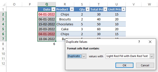
Click OK & one can see that all the duplicate cells have been highlighted as shown below.
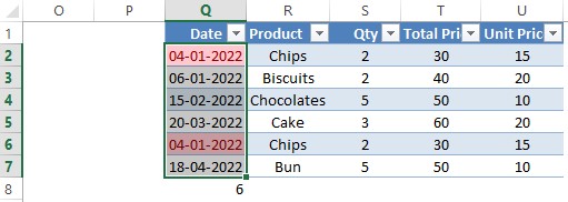
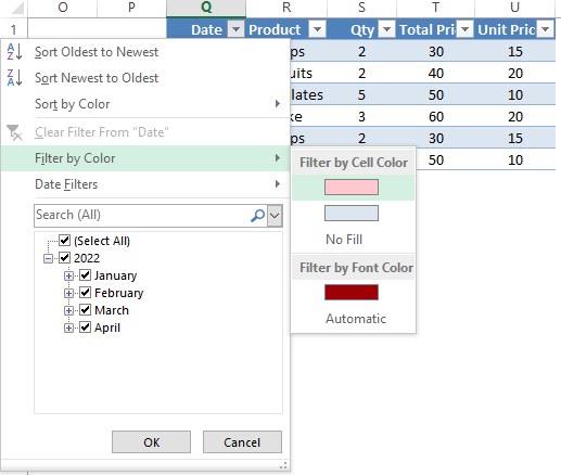
Now back to the question on which colour to filter, filter for this red colour & the count of duplicates will be automatically displayed below the bottom-most entry of the column.

Conclusion
Hope the article was informative. Do have a look at this article, to know how to count a range of cells using MS Excel. QuickExcel also has numerous other articles, which could help you in many ways to use MS Excel. Cheers!
