There are multiple reasons why you would like to compare columns in Excel. Though you can always compare manually this might get extremely difficult when dealing with and computing large data sets.
In Excel, you can either get the result of the comparison in the default ‘true‘ and ‘false‘ output or a custom output, meaning like anything ‘match’, ‘success’, ‘identical’, etc.
Also read: The Ultimate Guide to Sorting Data in Excel?
Compare Columns in Excel – A Basic Example
Let’s start with a simple example and compare columns in Excel where the row is the same. This becomes an easy start for even those who have never worked with formulas.
Default Output:
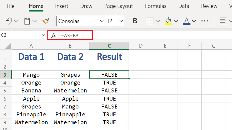
- To perform comparison as shown in the above image, apply the simple formula:
=A{n}=B{n}
where A{n} signifies the cell location and n=row number.
This default method of comparison gives output in the default value only – “true” or “false”
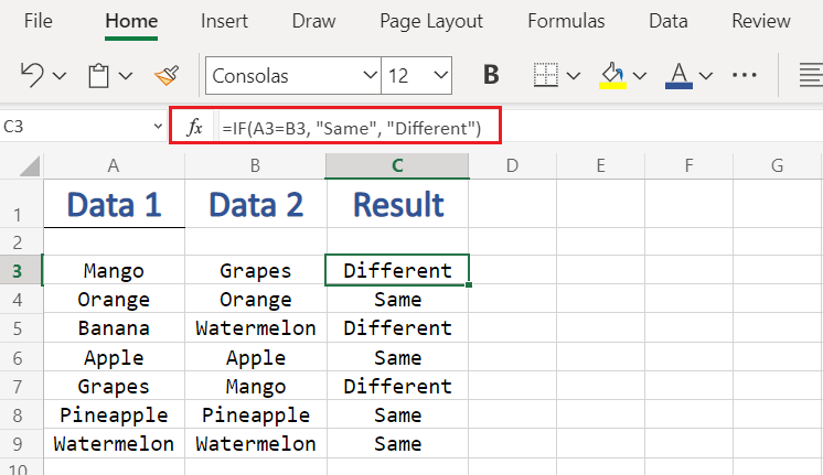
Custom Output:
To get a “Custom Output” from the comparison, we need to use the if function:
=IF(logical_test, [value_if_true], [value_if_false])
where:
A logical test can be anything A=B, A<B, A>B, etc.
[value_if_true] can be set to anything like “Same”, “Correct”, “t”, etc.
[value_if_false] can be set to anything like “Different”, “Incorrect”, “f”, etc.
To understand better, consider our below example of comparison of two columns:
Compare Two Columns and Highlight Matching Data
- Go to ‘Home’ inside an excel workbook.
- Select the cells which you want to compare and highlight by left-clicking and dragging to select.
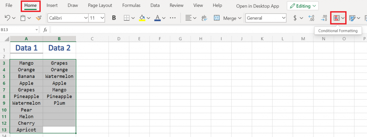
- Click on ‘Conditional Formatting‘ option which will further open a drop-down menu
- In the menu go with ‘Highlight Cell Rules‘.
- Then again from the option menu, select ‘Duplicate Values‘

- After selecting ‘Duplicate Values‘ you will be served with a pop-up menu
- Here you can select from two options: ‘Duplicate’ or ‘Unique’
where:
Duplicate: targets the values (data) which are duplicate
Unique: when this option is selected, it targets the values (data) which are unique. - There is also an option to select the color for text and also for cell borders.

- Click OK to Highlight the duplicated cell values as shown in the below example image.
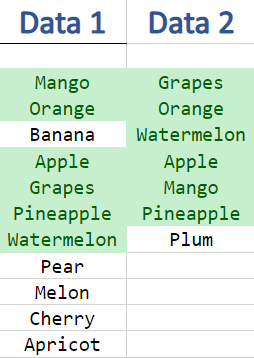
- To Highlight the cells which have ‘Unique Values‘:
- Under Conditional Formatting, Go to ‘Highlight Cell Rules’ to reveal a drop-down menu
- From the menu click on ‘Duplicate Values’ to reveal a pop-up menu
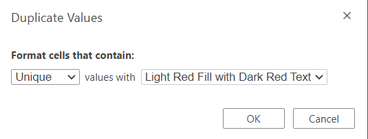
- From the menu select ‘Unique’ – under Format cells that contain [as depicted in above image]
- Click on OK to apply the highlighting.
Conclusion
And that’s it from our side. I hope you have learned well how to Compare columns in Excel and to highlight them. For more tutorials, stay tuned to QuickExcel!
