Clean data in Excel is a very important step before performing analysis on that data. It helps get rid of unnecessary and junk characters and helps maintain uniformity.
Also read: The Ultimate Guide to Sorting Data in Excel?
Different Ways to Clean Data in Excel
In this article, we will learn how to clean data using the following methods.
1. Remove extra spaces in Excel
The TRIM function in Excel removes spaces from the start and end of the text. It also removes extra spaces in between words except for single spaces. Syntax: TRIM(text), where text is the text or the cell reference to the cell containing the text from which you want spaces to be removed.
Let us consider two text examples, the first text contains extra spaces between the words and the second text has leading and trailing spaces.
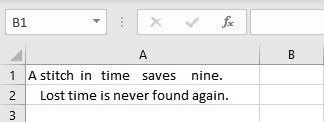
Follow these steps to remove extra spaces:
- Select the cell where you want to display the clean text.
- Type =TRIM(, select the cell containing the text and complete the formula with ).

- Press the Enter key to display the result.

- Copy the formula for the entire list by dragging down the fill handle.

2. Handle blank cells in Excel
Blank cells in a data set may result in error messages while using in-built functions in Excel.
Let us consider a data set of students with their marks, with marks of some students not available as they were absent. To handle such cases we may need to fill those blank spaces with the word Absent.
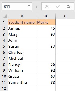
Follow these steps to find and fill the blank cells:
- Select the entire list which contains blank cells.
- Press the F5 key on the keyboard to launch the Go To dialog box.

- Click on the Special… button at the bottom left to launch the Go To Special dialog box.
- In the Go To Special dialog box, check the Blanks radio button and click on OK.
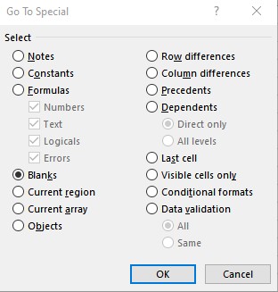
- All the blank cells are now selected, type Absent and press CTRL+ENTER to fill all blank cells with Absent.
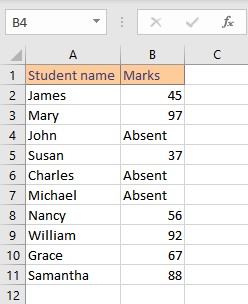
Note: If you simply press the Enter key after typing Absent, the value is inserted only in the current cell.
3. Change text case in Excel
Follow these steps to properly format names in Excel:
- Select the cell where you want to display the properly formatted names.
- Type =PROPER(, select the cell containing the text you want to format and complete the formula with ).
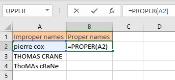
- Press the Enter key to display the result.
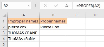
- Copy the formula for the entire list by dragging down the fill handle.
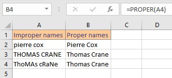
Improperly formatted emails are difficult to read, having all the letters in lower case make it easier to read. Follow these steps to properly format email addresses:
- Select the cell where you want to display the properly formatted emails.
- Type =LOWER(, select the cell containing the text you want to format and complete the formula with ).

- Press the Enter key to display the result.

Some words need to be written in all capital letters so that more emphasis is given to them. Follow these steps to properly format company names:
- Select the cell where you want to display the properly formatted company names.
- Type =UPPER(, select the cell containing the text you want to format and complete the formula with ).

- Press the Enter key to display the result.

4. Remove duplicates in Excel
Duplicate data may result in redundancy, cause calculation errors, and large file sizes. Follow these steps to effectively remove duplicates in Excel:
- Select the cells you want to check for duplicate values.
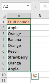
- Click on Remove Duplicates in the Data Tools group on the Data tab.

- Select the columns from which you wish to remove duplicates from the Remove Duplicates dialog box that appears and click OK.
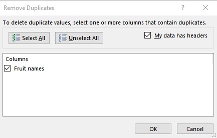
- A popup appears that tells us how many duplicate values were found and removed, and also the number of unique values that remain. Click OK.

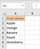
The final result looks like this:
5. Split Data into Columns in Excel
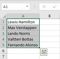
We can parse people’s names into first names and last names by using Text to Column functionality in Excel. Follow these steps to split data into columns:
- Select the cell containing the text you want to parse.
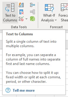
- Click on the Text to Columns option in the Data Tools group on the Data tab.
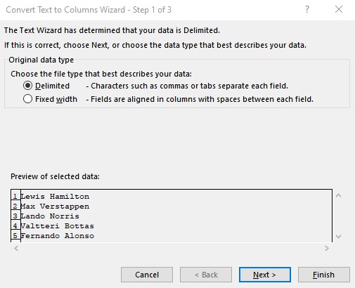
- In the Convert Text to Columns Wizard – Step 1 of 3 dialog box, check the Delimited radio button and click on Next.
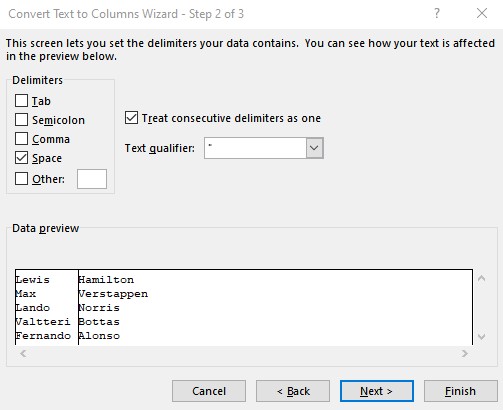
- Then in the Convert Text to Columns Wizard – Step 2 of 3 dialog box, check the Space check box under the Delimiters group and click on Next.
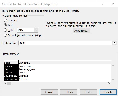
- Finally, in the Convert Text to Columns Wizard – Step 3 of 3 dialog box, check the appropriate data format radio button under the Column data format group and click on Finish.
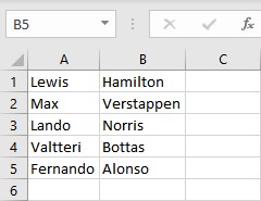
The final formatting looks like this:
Conclusion
In this article, we learned how to clean data in excel for data analysis.
