Rather than being a mere repository of numerical & textual data, MS Excel also serves as a vital tool to analyse those data with the aid of its in-built formulae. In this article, we shall look in detail at the sequence of steps that ought to be followed to create any formula in MS Excel.
Also read: How to Hide Formulae in MS Excel?
The Syntax:
The very first thing one has to get familiar with, before constructing any formula is the syntax of the formula. A syntax gives a generic outline of what the formula needs in order to compute the intended results from the data fed.
These constituents of the formula within its syntax are its basic constructs & it is imperative that any formula is started with an equals sign (=).
Without the equals sign (=) what might happen is that MS Excel does not get to know that there are some computations needed to be done & would treat whatever entries in the cell as regular data. So, never forget the equals sign!
Let us now have a look at the below syntax which depicts in general the constituents of any formula.
= formula (instruction_1, instruction_2,……..)
Where,
- formula – name of the formula such as SUM, PRODUCT, IF, VLOOKUP & so
- instruction_1, instruction_2 – commands or conditions which need to be satisfied for the functioning of the formula
Listed below are some examples which reflect the above depiction.
=SUM(number1, number2, ……….)
Where,
- SUM – formula used to add the numbers within the selected range
- number1, number2 – references to the cells with the numbers or numbers directly entered within the formula
- (………) – round parentheses which denote the start & end of the formula
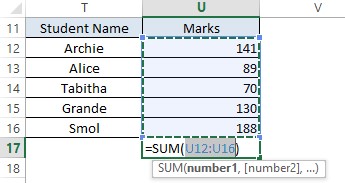
Here is the SUM formula in action!

It can be observed that all the cells are not given as (U12, U13, U14, U15, U16) within the formula, but rather referred to as (U12:U16). The colon sign between these two cells indicates that all the cells that fall within the start & end cell addresses given are selected to perform the operation for which the formula is called.
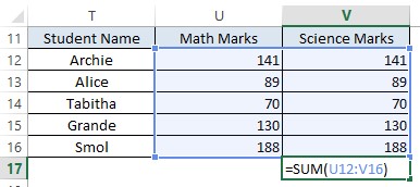
This also holds good when the reference is given as (U12:V16) which selects all the cells between the start cell U12 & the end cell V16 as shown below.

The Operand Formulae:
While all formulae start with an equal sign (=), some formulae don’t fall under the syntax depicted above. These are known as the ‘Operand Formulae’ and their syntax can be portrayed as,
= number_1 [operand] number_2 [operand] number_3……..
Where,
- number_1, number_2……. – are numbers upon which an operation is to be carried out or references to the cells containing the numbers
- [operand] – a symbol which indicates the type of operation that is to be carried out
Following is the list of the commonly used operands in MS Excel,
- + Adding Operand
- – Subtracting Operand
- * Multiplying Operand
- / Dividing Operand
- ^ Exponential Operand
One has to bear in mind the BODMAS rule while using the above operands since formulae of this type don’t call for the explicit usage of the round parentheses.
BODMAS – Brackets of exponents, then Division, then Multiplication, then Addition & then Subtraction
What this means is that when all these or a combination of the above-given operands are used in a formula without the usage of round parentheses, then the sequence of computation will happen to start with the exponent & then with division & so on as stated above.
Let’s say we multiply 3 by the sum of 431 & 587 divide it by 7 & raise the result to the power of 2, the following formula might seem to be synonymous with the above requirement.

But if we include the parentheses to group the numbers according to the operations stated above, only then we shall get the correct answer. You can try it manually & verify just to be sure.

Conclusion:
Hope now you would be familiar with creating formulae in MS Excel. Here’s an article which elaborates on how to use $ within formulae in MS Excel. There are more cool articles in QuickExcel about the formulae in MS Excel, for you to catch up with ever-evolving trends. Cheers!
