Having a spreadsheet is all about dealing with numbers and in this article we are going to look into how to carry out one such arithmetic operation using MS Excel.
Enter MULTIPLICATION!
Let’s say you have purchased a list of items on different days and decide to use MS Excel to calculate the total expenditure. We would be covering two ways of carrying it out in this article.
- The Operand way
- The Formula way
We shall stick to the following example throughout this article.

So, what we have in hand is the price per unit of each item and also the total quantity of each item purchased. Now, let’s get on with the HERCULEAN task of computing the total amount spent on each item in each of the above-listed methods.
Method I – The Operand Way
Like all the formulae construction in MS Excel, the one which uses the operand too starts with an equal to sign “=” as shown below.
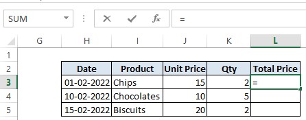
Click on the cells that are needed to be multiplied. In this case, we would first click on cell J3 which contains the Unit Price of Chips and cell L3 becomes like the one shown in the below image.
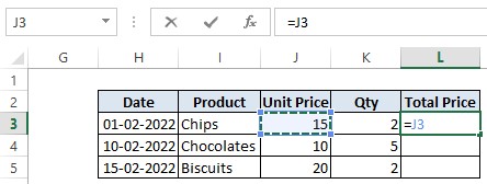
Now it is time to introduce the operand in place. The operand for multiplication in MS Excel is an asterisk (*). Similar to the conventional practice, here too we would be placing the operand in between two variables. In this example, there are 2 variables, viz. Unit Price & Qty.
So, after selecting the cell J3 which has the Unit Price enter the asterisk (*) as shown below.
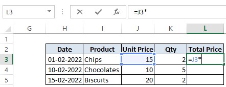
Once done, click on the next cell K3 which contains the Qty. of Chips. Now the cell L3 becomes similar to the one in the below image.

Press Enter key and voila! The product of the Unit Price and the Qty is now displayed.

It’s time now to deploy the formula to the other products as well. Click back on cell L3 and copy the formula in the cell by pressing CTRL+C.
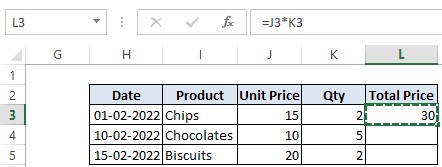
Now select the cells L4 and L5. Press CTRL+V to paste the formula on the selected cells so that the product of the Chocolates and Biscuits is also calculated.
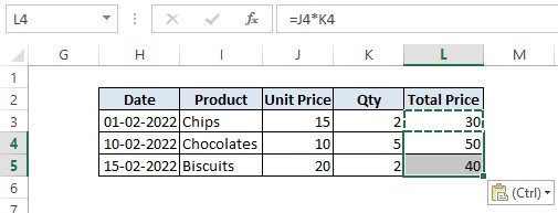
So now we have come across not only how to construct a formula using an operand, but also to copy and paste it to the other cells as well.
Method II – The Formula Way
Yet another way to multiply the desired numbers using MS Excel is by adopting its pre-defined formula. There are a variety of formulae in-built in MS Excel, but let us stick to the one which helps us to multiply for now. You can always check out other interesting posts on QuickExcel to know more about using MS Excel.
The particular formula of interest here is the one known by the term PRODUCT. In order to use any formula, it’s a mandate to start with an equal to “=” sign. The following is its syntax,
=PRODUCT (number1, number2, ……………)
What it means is, we can mention the number or the cell which contains the number we desire to multiply in the place of number1, number2, and so on.
Let’s apply this to the example we’ve taken in this article to see how it works.
We shall start with the equal to sign “=” followed by typing the term PRODUCT. Now, we open a bracket as shown in the following image.

Once done, we click on cell J3 containing the unit price of the product Chips and the contents of the cell L3 gets altered as in the below image.

After that, we would now include the Qty by clicking on cell K3 followed by closing the bracket.
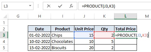
Press Enter & the product of both the Unit Price and Qty would appear in cell L3.

Now we shall repeat the same steps as in the closing of the previous method where we copy the contents of L3 and paste it on the cells L4 & L5.
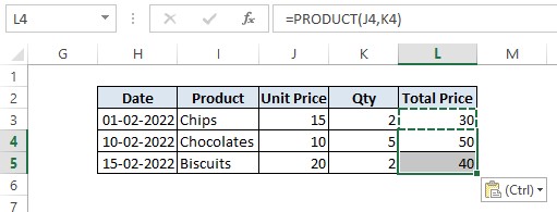
The products of all the entries in the columns J & K as in Unit Price & Qty, are now displayed in column L under the title Total Price.
Conclusion
Hope you have found it informative. We have covered the different ways to multiply in MS Excel in this article, but QuickExcel has numerous other articles which could help you with that one thing that you’re longing to do with MS Excel right now.
