In this tutorial, we’re going to learn to create a project timeline in Excel. We will also learn to customize timelines as we like.
Steps to create a timeline in Excel
Let’s begin to quickly create and customize a timeline with the help of this step-by-step tutorial.
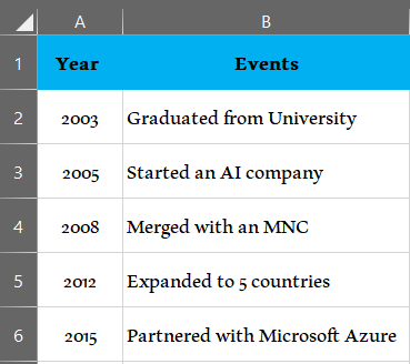
Before creating a timeline, you can either have a table of events prepared to render data into the timeline from it, or you can choose to create a timeline first and then add events to it later.
Let’s get started!
- Open a blank Excel file.
- Select anywhere in the cell range if you have an event table already prepared.
- Go to the Insert tab.
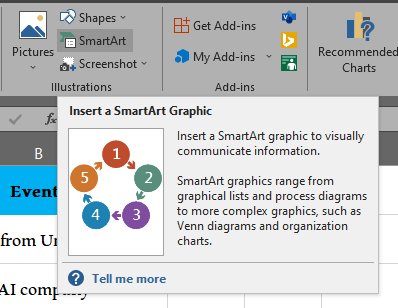
- Click on SmartArt in the Illustrations section.
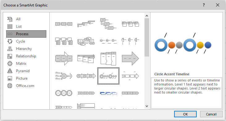
- A window named Choose a SmartArt Graphic opens.
- Click Process on the left side.
- Scroll down and select the Basic Timeline or Circle Accent Timeline.
- We have selected the Circle Accent Timeline for better understanding.
- Click OK to continue.
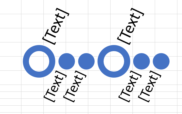
You can now see that a circle accent timeline has been inserted in the sheet. But you can see that the events have not been named yet.
Let’s begin adding events to the timeline.
- Click anywhere in the timeline area.
- Press CTRL+A to select all the text boxes.
- Go to the Design tab.
- Click on Text Pane in the Create Graphic section.
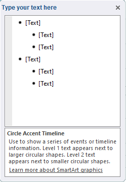
- Click on one of the text boxes in the Text Pane window.
- Press CTRL+A again to select all text boxes.
- Copy (CTRL+C) the year and the events from the event table and paste (CTRL+V) in the text pane.
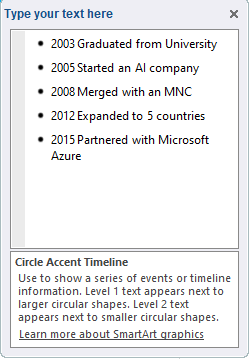
You can see that the text from the table is pasted to the text pane.
Also read: How to Add Bullet Points in Excel?
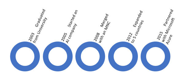
You can see that the text added in the text pane is being displayed in the timeline.
- If you want to separate events occurring in the same year, press TAB on your keyboard to add an event under the main event.
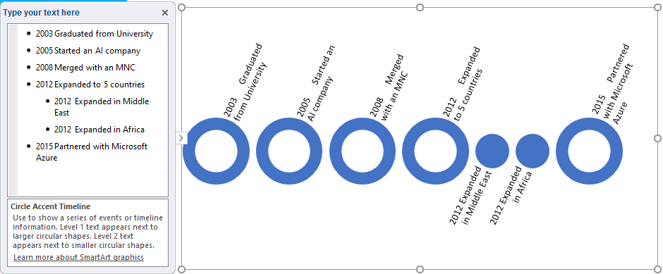
You can see that two sub-events have been added to the timeline for the year 2012.
Customizing timelines in Excel
Let’s begin customizing the timeline in Excel. To change the style of the timeline, follow these steps.
- Click on the timeline.
- Go to the Design tab.
- Pull down the box under the SmartArt Styles section.
- Select a style that you like.
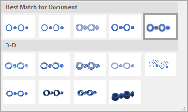
Take a look at this new style that has been applied to our timeline.
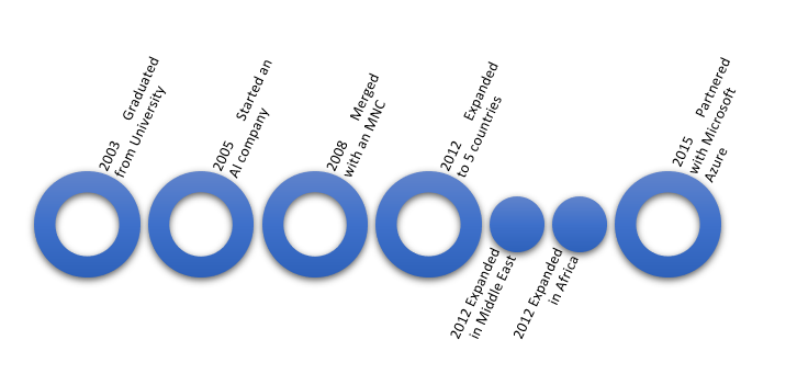
To change the layout of your timeline, do as follows.
- Click on the timeline.
- Go to the Design tab.
- Under the Layouts section, pull down the box to view layout styles.
- Select a layout that you like.
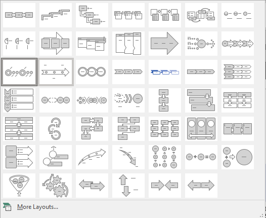
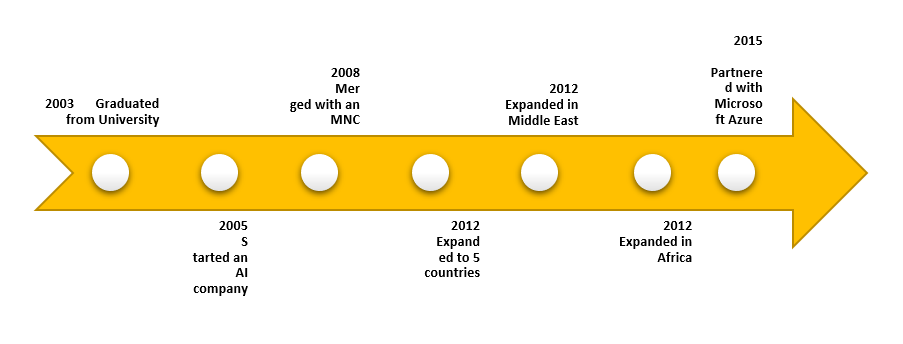
We have selected the Basic Timeline to change the layout.
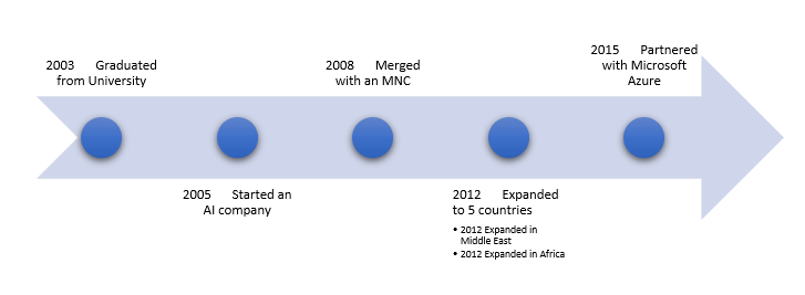
But the limitation of this timeline layout is that the secondary events do not separate properly. You have to add each sub-event and main event as the main event in this layout.

You can see that we have converted sub-events to main events to fit in this layout.
To edit the text in a timeline, do as follows next.
- Go to the Design tab and click on Text Pane.
- Press CTRL+A on your keyboard to select all texts in the box.
- Go to the Home tab.
- Choose a font color, font size, and text formats like bold, italics, or underline.
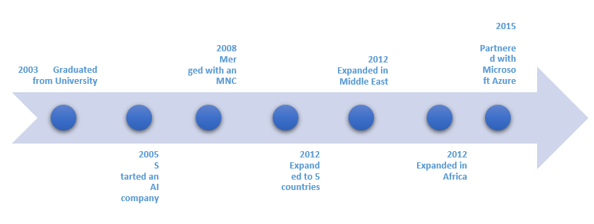
You can see that the texts in the timeline have been customized.
To change the color of the accent, follow these steps.
- Click in an empty area in the timeline.
- Go to the Design tab.
- Click on Change Colors.
- Select a color combo you like for your timeline.
- Note that choosing a color combo from this option will change the text colors applied by you previously and will be adjusted as per the color scheme you selected.
Take a look at the new color scheme applied to the timeline.
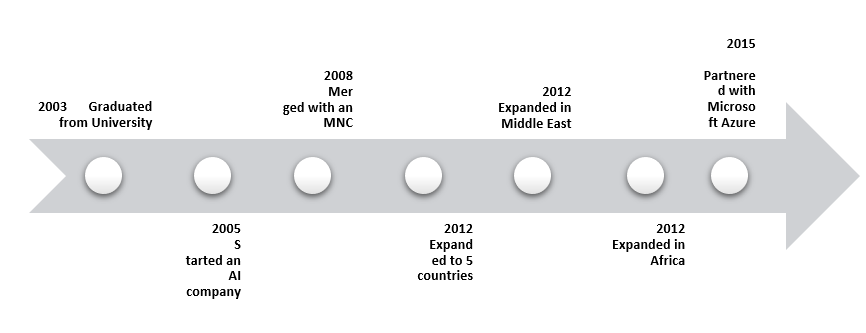
To change the color of the accent’s arrow, do as follow.
- Click on the arrow.
- Go to the Format tab.
- Under the Shape Styles section, select your favorite color and style by pulling down the box.
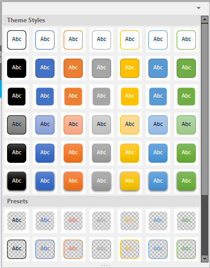
Take a look at this new shape style applied to our timeline.
Conclusion
This was all about creating and customizing timelines in Microsoft Excel. Feel free to comment below if you have any doubts regarding timelines in Excel.
