In this tutorial, we will learn about the IF function in Excel. Along with IF, the AND and OR functions are important formulas too. A nested IF simply means multiple IF functions in a single syntax.
Introducing IF Function in Excel
Let’s get started with this easy guide to using the IF function and all its related functions in Microsoft Excel, step-by-step with supporting images and examples.
1. IF Function
To learn to use the IF function, we will take an example of a mark list of students below.
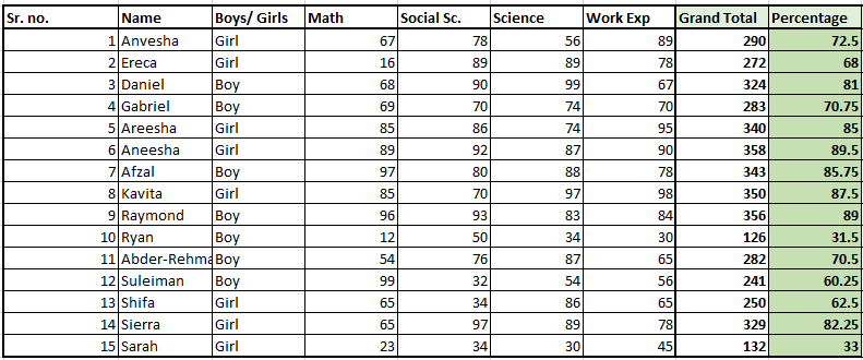
Our goal is to find out which student has passed or failed and what are their grades. Of course, it would be a tedious task to find out pass or fail results and grades for each student in this list.
To ease our task, we have IF functions for that matter. The IF function will automatically identify if a student has passed or failed based on the criteria you provide to it.
It will automatically mark a student as “Pass” if he/she has scored above the minimum pass mark and mark a student as “Fail” if he/she has scored below the minimum pass mark.
The IF function automatically assigns the appropriate grades to students based on their marks if you command it.
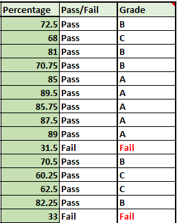
Here is a glimpse of how the IF function helps you out with assigning grades and marking “Pass” or “Fail”.
Steps to use IF function in Excel
We have allotted certain grades and marked them as Pass or Fail to students based on the percentages they have secured in their exams, with the help of the IF function.
1. Using the IF function in Excel to identify passed/failed students
Let’s learn how we can use the IF formula to achieve this. We will use the same example. We take the minimum passing percentage as 34%.

- Find out the percentage of total marks of every student.
- Create a new column named “Pass/Fail”.
- In the blank cell below the title, type the IF formula as follows next.
- Type =IF( and select the first student’s percentage and type >=34.
- Put a comma and move to the next argument named [value_if_true]. This means you’re being asked to put a value to be displayed if the above condition is true. Remember these arguments are case sensitive.
- Once you have put a comma, type “Pass”.
- Put a comma and move to the next argument named [value_if_false] to display a value when the above condition is false. This field is optional in most cases but we need a false value because it is a mark list.
- Close the bracket and hit ENTER.
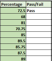
You can see that the formula is displaying “Pass” for the first student because she has secured above 34%.
- Double-click or drag the cell from the right corner below to autofill the formula to all the students below.
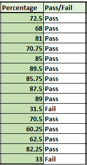
Recommended read: How to Autofill in Excel?
2. Nested IF Function
Now, let us start assigning grades to all students.
We are going to be using multiple IF functions in a single syntax this time to provide multiple criteria to the IF function. This is called Nested IF in Excel.
However, there is no specific function named “Nested IF” in Excel, it is simply that this behavior has been given a name i.e., Nested IF.
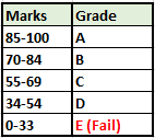
Before we proceed further, we need to first make a table that displays a grading class for each grade. Here is an example below.
- Create a new column named “Grade”.
- Type the IF function in a blank cell below the title as follows.
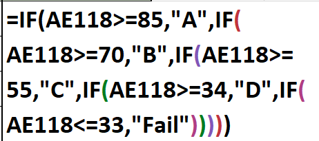
- Type =IF( and now type AE118>=85,”A”,IF(AE118>=70,”B”,IF(AE118>=55,”C”,IF(AE118>=34,”D”,IF(AE118<=33,”Fail”.

- Note that AE118 is our cell address for the first student’s percentage. It will be different in your case. Refer to the image above to make sense of the formula.
- The formula simply states- if percentage marks are above and equal to 85 then give “A”, if percentage marks are above and equal to 70 then give “B”, and so on and so forth. For the last condition, we have applied the condition- if the marks are less than or equal to 33 then give “Fail”.
- For the last IF statement, you can either put the result as “Fail” or “E” as you like.
- Now, note that we will close the formula with 5 brackets for this example as we have used a total of 5 IF formulas.
- Hit ENTER to complete the formula.
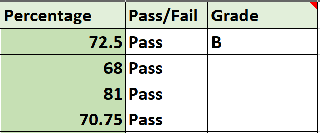
You can now see that the formula has been applied to the first entry and the result is B because the student has secured 72.5% which is less than 75%. This means the nested Ifs are working correctly.
- Now drag the cell from the lower right corner to autofill the formula to the rest of the entries.
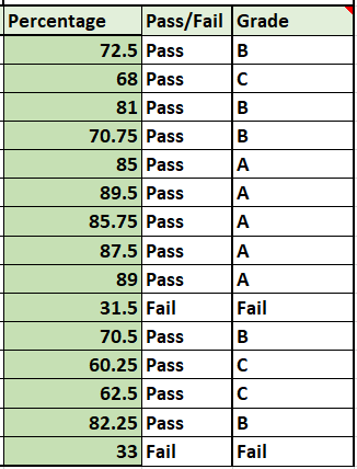
You can see that we now have grades and pass/fail markings for every student on the list successfully.
3. IF with AND in Excel
Let us learn the IF formula with the AND function in a single syntax with a minor example.
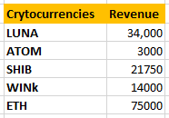
When you have two or more distinct conditions to be used together, you can use the IF function with AND in Excel.
While nested IFs will also work, using AND function will save your time as it is shorter to type. So, let’s get started.
Our goal is to identify currencies with revenues greater than 20,000 and less than 50,000 and mark them as “Good”.
- Type =IF(AND( because we are using the IF with AND function.
- Select the first cell under Revenue, and type >20000.
- Put a comma and select the first cell under Revenue again and type <50000.
- Now, close the bracket to complete the AND function. We’re still working on the IF function so do not put two brackets.
- We come back to the IF function as soon as we close the AND function. Now put the values to be displayed if the condition is true or false.
- Put a comma to move to the argument [value_if_true] and type “Good”.
- You can provide a result in the [value_if_false] argument, but it is completely optional. If nothing is provided then the cells will display FALSE if the condition is false. But if you want the cells to remain blank simply put “” (two double quotation marks) in this argument.
- Close the bracket to complete the IF function as well.

This is how the syntax should look like before pressing ENTER.
- Hit ENTER to view results and drag the cell down to autofill the formula to the rest of the cells.
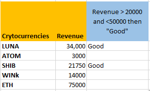
There are only two such cells for which the condition is true and the result is being displayed as “Good” for them and the rest of the cells are blank. This means the formula is working correctly.
4. IF with OR in Excel
Using the OR function with the IF function will give results for either of the conditions that are true.
- Type =IF(OR(.
- Select the first cell under Revenue and type >=20000.
- Put a comma and select the first cell under Revenue again and type <=50000.
- Now, close the bracket to complete the OR function. We’re still working on the IF function so do not put two brackets.
- Coming back to the IF function, we now put the values to be displayed if the condition is true or false.
- Put a comma to move to the argument [value_if_true] and type “Flag”.
- Put a comma to move to the argument [value_if_false] and type “”.

This is how the syntax should look like before pressing ENTER.
- Close the bracket to complete the OR function and hit ENTER.
- Drag the cell below to get the results for the rest.
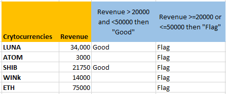
The formula is true for all entries and so it is displaying “Flag” for all of them. This is because all the values are either lower than 50,000 or greater than 20,000.
Conclusion
This was all about IF functions and other related functions to the IF function that are AND and OR functions.
Reference: ExcelJet
