You can shade alternate rows to make the data in your worksheet easier to scan and soothing to the eyes. This is also known as color banding. In this article, we will learn how to shade every other row in Excel.
Also read: Select non-adjacent cells in Excel
Here’s the step to step guide to shade alternate rows in Excel
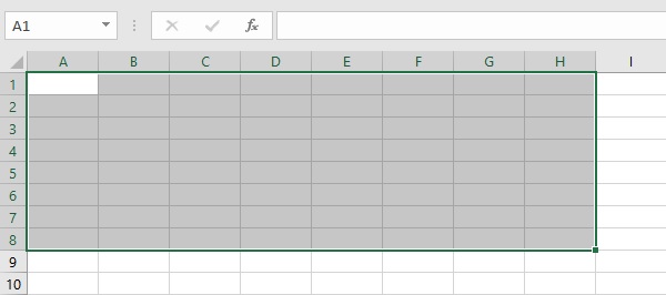
- Select the range of cells that you want to format.
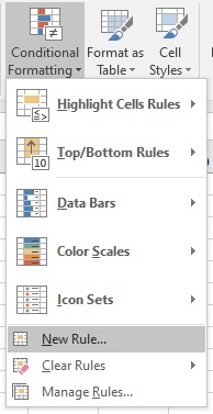
- Click on Home > Conditional Formatting present in the Styles tab.

- Select New Rule from the drop-down list.
- In the Conditional Formatting dialog box, click on Use a formula to determine which cells to format option present in the Select a Rule Type section.
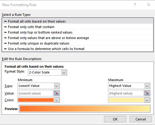
In the Format values where this formula is true box, type the formula:
- =MOD(ROW(),2)=0 for shading even numbered rows or
- =MOD(ROW(),2)=1 for shading odd-numbered rows.
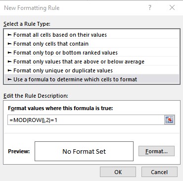
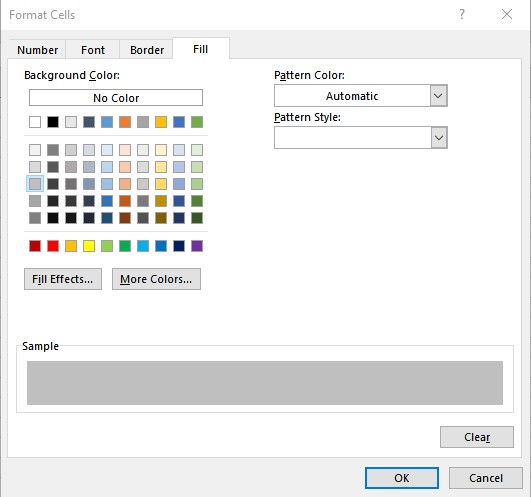
- Then click on the Format button to open the Format Cells dialog box.

- Click on the Fill tab to select a color for shading. After selecting the color click on OK.
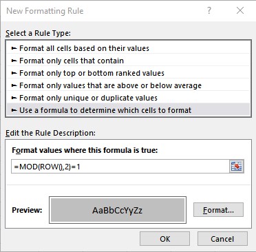
- After seeing the preview in the Conditional Formatting dialog box, click on OK, to apply the shading.
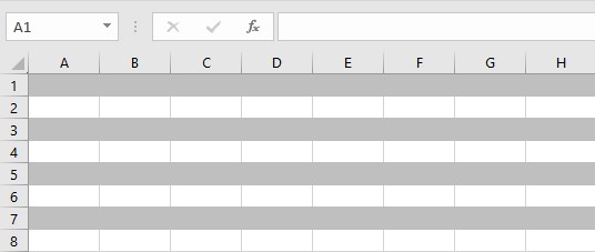
The final result looks like this:
Conclusion
In this tutorial, we learned how to shade every other row in Excel using Conditional Formatting.
