Welcome to Part 2 of creating a searchable dropdown list tutorial in Excel. If you’re new here and want to learn to create searchable dropdown lists from scratch in Excel, then read part 1 of this guide first.
This guide is for those who are on an older version than Office 365 and want to make searchable dropdown lists without using the FILTER and UNIQUE functions in Excel.
Let’s carry on with part 2!
Using the OFFSET and COUNTIF functions
Once you have hidden the N/A errors using the IFERROR function, the next step is to use the OFFSET formula to be able to automatically select the search terms that appear when searching. These selections will then be inserted in a dropdown list further.
Here are the further steps.
- Click on a blank cell adjacent to the cell with the VLOOKUP function and other functions in it.
- For the first argument, that is, reference, select the first cell with the VLOOKUP and other functions.
- Press F4 or Fn+F4 and lock the cell address.
- Put three commas together because we do not need to provide the rows and columns.
- For the height argument, enter the COUNTIF formula. Type COUNTIF(
- Now, select the entire column range with the VLOOKUP and other functions.
- Lock the former cell address of the selected column range.
- Put a comma, and type “?*”))
- Hit ENTER
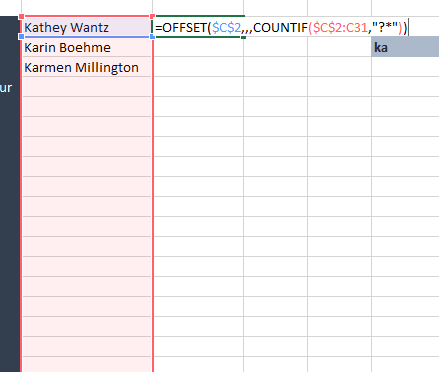
The ?* denote text values in Excel. So, Excel will count cells if there are any text values in them.
You will see the first name is displayed in this cell now.
Now, the next step is to name the formula you just wrote.
- Click on the cell with the OFFSET and COUNTIF formula.
- Copy the formula from the formula bar above. CTRL+C to copy.
- Go to the Formulas tab.
- Click on Define name.
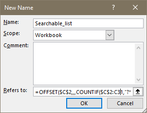
- Enter a custom name. Make sure to add an underscore instead of spaces in the name.
- Remove the existing formula in the Refer to the field and paste your formula here.
- Click OK.
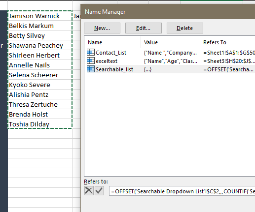
Now, your selection will expand according to any number of entries that display in the column. You can check this by clicking on the Name Manager button in the Formulas tab.
The next and the most interesting part is creating the dropdown list. Let’s get started.
- Click on the search box cell where you will create the dropdown list.
- Remove anything written in the search box.
- Go to the Data tab.
- Click on Data Validation.
- In the Settings tab, select List.
- Click in the Source field and press F3 or Fn+F3 on your keyboard.
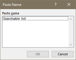
- Choose the name of the formula you just created.
- Click OK.
- Click OK again.
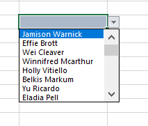
You now see all the names in the dropdown list below the search box.
But, there is a problem here. You have to enter the full name of the person you are searching for from the list. Otherwise, you see an error message.

This error message was displayed when we tried searching for the term “Ka”.
Let’s solve it quickly!
- Go to the Data tab.
- Click on Data Validation.
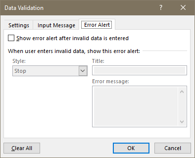
- In the Error alert tab, uncheck the box.
- Click OK.
Try searching for that term again and pull down the list.
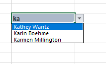
You can see that we can see only those names that have “ka” in them.
Woohoo! You now know how to create a searchable dropdown list in Excel!
Time for a coffee break!
Conclusion
This tutorial was the final part of creating a searchable dropdown list in Microsoft Excel. We recommend you to read part 1 first to learn to create a searchable list from scratch in Excel. Stay tuned for more fascinating topics like this!
