Things don’t really happen, the way we want them to. The same holds true for MS Excel too where there can be an unprecedented turn out of events even with the slightest change. Additional spaces within the contents of the cell are a real pain! They find their way in when data is being downloaded as an Excel file or copied from some other source into an Excel file or sometimes due to the oversight while entering data manually.
However, MS Excel being always nice to its users has found a way to keep this excessive evil in check. In this article, we are going to explore how to remove the unnecessary additional spaces within the contents of the cells.

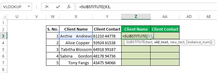
In the above data, it is visible that someone has really played around with the spacebar while recording the client names. Also, it can be seen that their contact numbers have also been separated by a space in the middle. Let us say, that we have a requirement where both the client names and the contact numbers are needed without any spaces between them. There’s a formula waiting backstage just for this occasion.
Remove spaces using the SUBSTITUTE formula
A SUBSTITUTE formula has a self-explanatory function using which one can replace a certain portion of a cell’s content with those which are desired. Following is the syntax of this formula,
=SUBSTITUTE(text, old_text, new_text, [instance num])
As always the EQUALS (=) sign alerts MS Excel that there’s a formula coming up so that it preps up all the relevant built-in features ready for deployment. This when followed by typing the word SUBSTITUTE limits those features to the line of instructions relevant to this particular formula.
Let us decode those instructions within the brackets now!
- text – Entire contents of the selected cell
- old_text – The portion of the text that needs to be replaced
- new_text – The text that is to substitute the old text mentioned previously
- [instance num] – Which specific occurrence of the old text is to be replaced? The first or second & so on. If not selected, all occurrences are replaced with the next text.
Now, we shall start constructing a formula to remove all the spaces from the entries under the Client Name column. Once, the SUBSTITUTE formula is put in place, the required cell is selected in the place of ‘text’ given in the formula’s syntax as shown below.

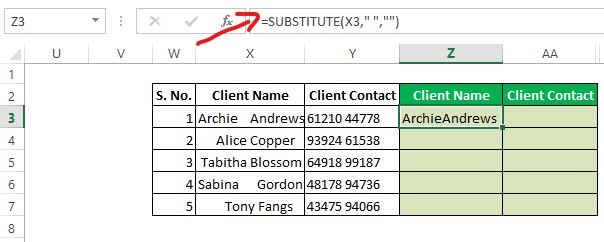
We are in for a bit of a trick now! What we are trying to get rid off are all the spaces within the contents of the cell. So, we leave a space between two double quotes as shown below.

Why the double quotes? – one might think. That’s the only way to put a text within a formula in MS Excel. Without these double quotes, references to any text by simply typing them within the formula don’t work.
The next step is to put the text that would replace the space. So, what would that be?
NOTHING! We don’t want the spaces, which means we don’t want anything in that place. We carefully convey this to the SUBSTITUTE formula again with the help of the double quotes by leaving no space in between them as shown in the below image.

Once done, the closing bracket is included to conclude the formula. It can be seen that we have not given our attention to the [instance_num] part, since here we want to remove all the spaces there are & by default the SUBSTITUTE formula does just that.

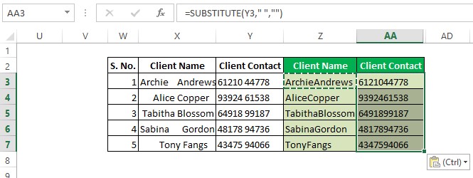
Likewise, the same formula can be copied using CTRL+C or right click, Copy and then pasted throughout the other cells too to obtain the results as shown below.

Conclusion
Since the formula would auto-adjust their cell references to the cells where they are pasted, it won’t be necessary for us to construct the formula again for the Client Contact in Column AA. Hope this article was informative. QuickExcel also has numerous other articles, which could help you in many ways to use MS Excel. Cheers!
