We would have successfully tabulated a list of data under a range of column headers. But, there might be instances when we would be needing to move certain rows from the position where they are to some other place within the active sheet. Not all the time, but sometimes we’d face this situation and in this article, we would be covering the ways to handle just that.
Listed here are the different ways of having it done.
- The Move Method
- The Overwrite Method
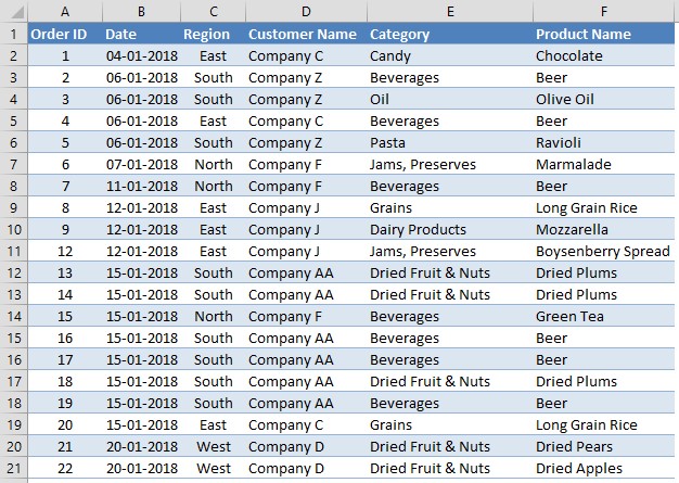
We would be trying to move the rows in the following table using each of the above-listed methods.
Also read: [Easy] How to find and remove duplicates in Excel?
1. The Move Method
At the very first, we need to select the row which we need to move. This can be done by clicking the leftmost cell of that row which would be under column A & selecting the other corresponding contents by dragging the cursor towards the left.
Oops! Didn’t I mention this first? All this needs to be done without lifting that finger pressing the left mouse button.
Once that is done, hover the mouse over the selected contents till the time, the cursor turns into the following symbol – a cross with arrows at all the ends.

Here’s how the cursor would look upon reaching the right spot over the selected contents.
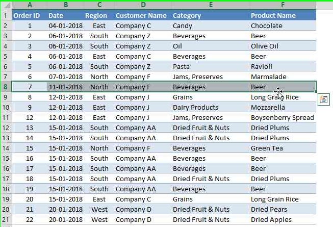
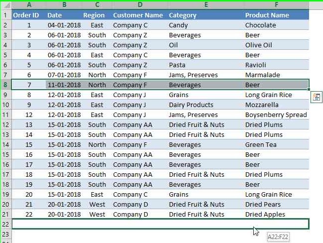
Click on the very spot where the cursor changes into the above symbol and drag the contents to the desired location. In this case, let’s say, we would like to have it at the bottom of the tabulation. So, we would drag until it reaches the very bottom.
In the below image, it can also be seen that the destination address to which the contents are to be placed also appears alongside the cursor. In this case, it would be from the cells A22 till F22, and the same is displayed as A22:F22, with the colon ‘:’ indicating that it contains all the cells between those mentioned on either side.
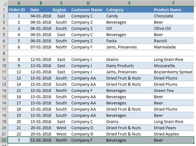
Once the cursor reaches the destination location, lift the finger off the left mouse button and the contents would be moved to that very place in no time.
2. The Overwrite Method
The very first step where we would select the contents and place the cursor where it changes to move the contents remains the same as in the above method.

On the other hand, this method would only be used once we would like to replace the contents in a set of data with something which we already have.
Let’s say, we would like to replace the contents of row 10 in the above tabulation with those from row 8.
Click on the part where the cursor changes into the cross symbol with arrows at all the ends with the left mouse button & drag the selected contents until it reaches row 10, without lifting that finger off the button.
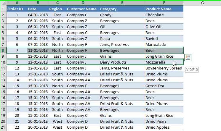
Once the cursor reaches row 10, lift the finger off and the following pop-up will appear. This can also be cross checked with the cell address that would be displayed alongside the cursor. In this case, the displayed address should match with A10:F10.
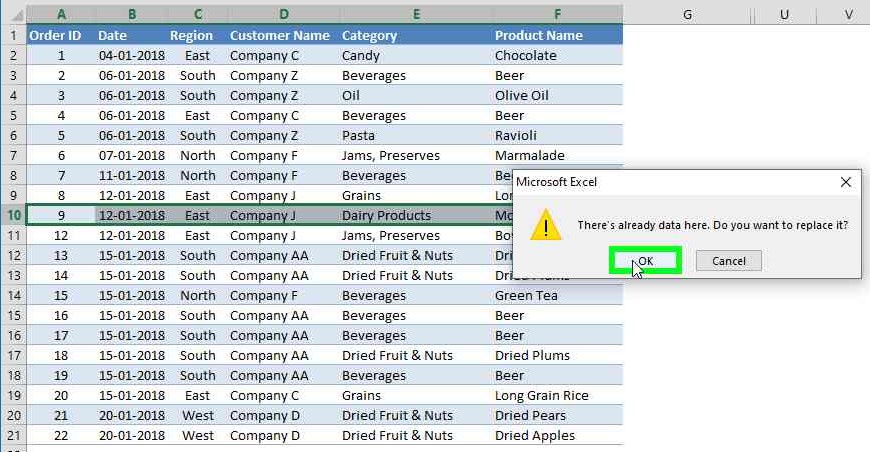
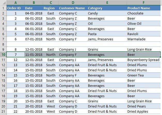
Click OK & the original contents in row 10 would be replaced in a whiffy!
Conclusion
That’s the end of this article. Hope now you would be familiar with the different ways to move the rows within the active sheet. For much more tips and tricks on using MS Excel, please do look into our space QuickExcel. Until then, Cheers!
