Ever delegated the task of compiling data to someone and got it back with some misplaced entries? It would be needed to shift some entries down in order to insert the correct data at the correct place. There might be a couple of ways to go around that & we would cover both in course of this article.
Here are the different ways of shifting the cells down,
- Using the Keyboard Shortcut
- Using the Home Tab
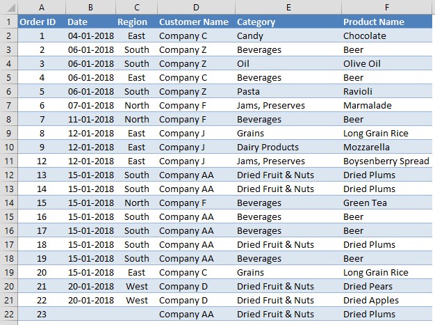
We would be trying to shift the cells, as in those of the columns B & C of the following table using each of the above-listed methods.
1. Using the Keyboard Shortcut
In the above table, it is evident that there is a missing entry for the Date & Region, in row 22. Let’s say that the Date & Region entries for rows 20, 21 & 22 are misplaced one cell upwards. What this means is that the entries for row 19 are incorrect.
So, a viable option here is to shift all the existing entries in columns B & C from row 19 till 21, one cell downwards.
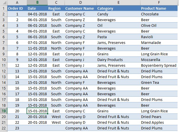
In order to do this, as always we would be needing to select the cells by using the left mouse button to click on the leftmost cell of the selection as shown in the below image.
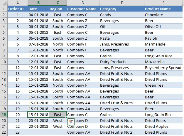
Once done, without taking the finger off the left mouse button drag the cursor down till it reaches cell C19.
Now comes the part of interest! Your attention, please!
Hit the CTRL key followed by pressing the SHIFT key and then press the Plus ‘+’ key. The emphasis here is to press the keys one after the other and NOT SIMULTANEOUSLY. Doing the latter would only put this method in vain.
CTRL + SHIFT + PLUS (+)
The successful execution of the above step can be validated upon the appearance of the following pop-up. This pop-up contains a list of options to choose from, each proposing a different outcome on what could becometh of the selected cells.

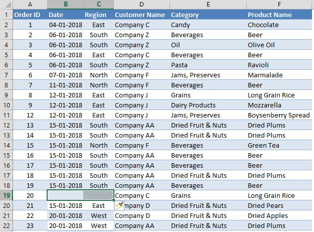
Click on the Shift cells down option to shift all the selected contents one step down and then click OK. The selected contents and also those which are immediately below would then be shifted one cell downwards, leaving cells B19 & C19 blank for us to enter the right details.
2. Using the Home Tab
The initial steps involving selecting the misplaced contents remain the same as stated in the above method. It’s only during the shifting cells down part, this method varies and we shall see how!
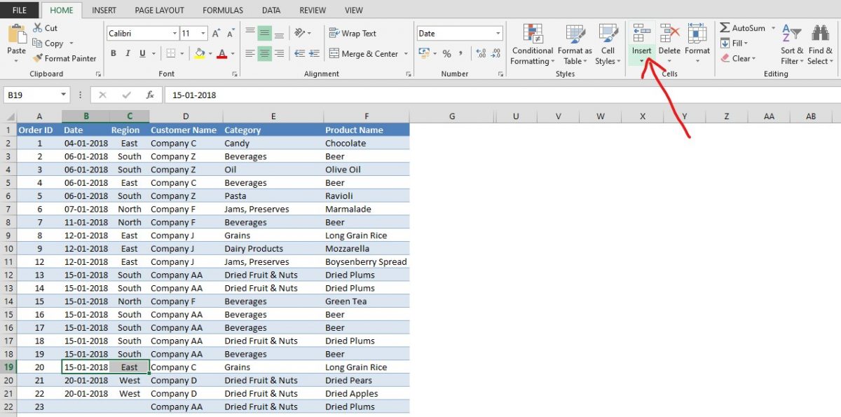
After selecting the required contents as shown in the below image, click on the Insert option seen under the Home tab.
A list of options to choose from would now appear as shown below.
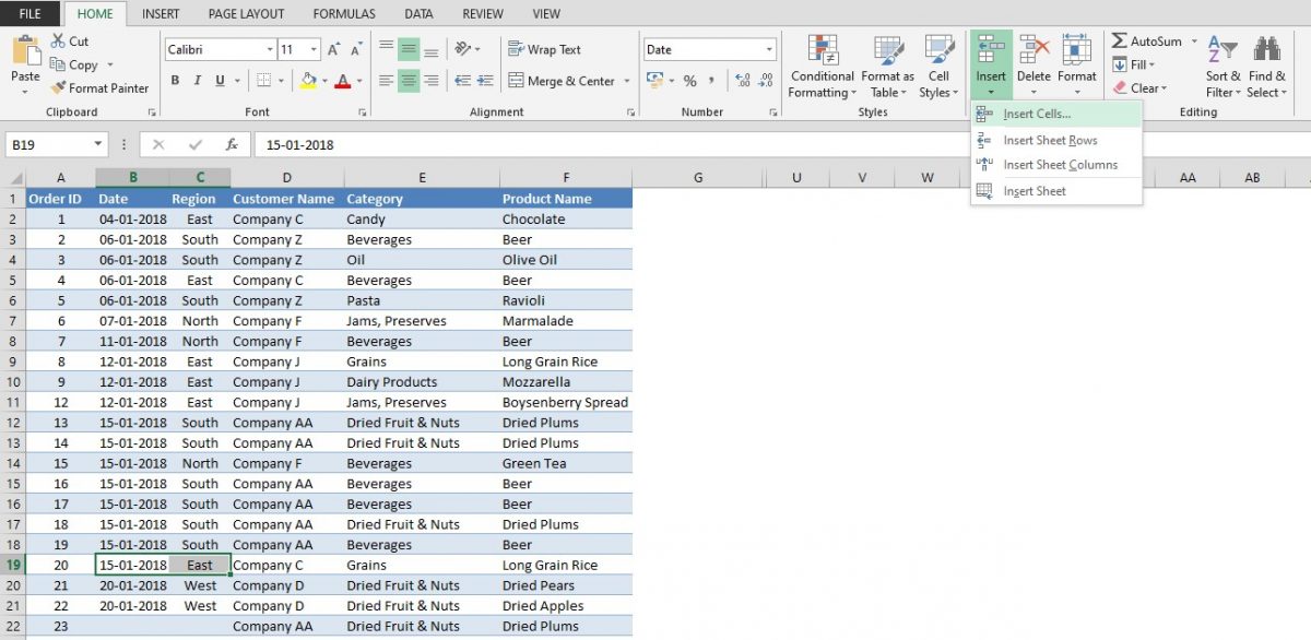
Click on the Insert Cells option and a pop-up would appear.
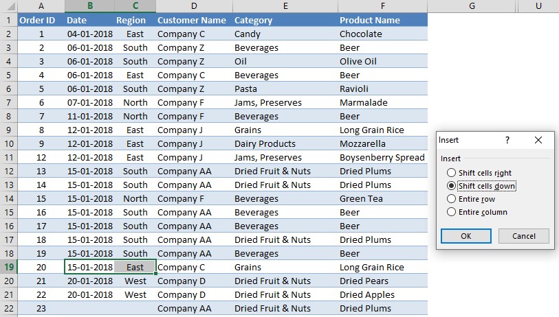
Select the Shift Cells Down option and click OK. The contents from row 19 till 21 in columns B & C would be shifted one cell downwards.

Conclusion
Now that we’ve covered 2 different ways to hide the cells in MS Excel, hope it would come in handy when you face a situation of need. This article has predominantly dealt with shifting a selected group of cells downwards. But, there shall also arise a need to move an entire row. That being said, check out this article, if you want to move an entire row in an Excel sheet. Do watch out for our space, QuickExcel to keep yourself updated with MS Excel. Cheers!
