Merging 2 cells doesn’t pose much of a hassle. Select both cells and click on the Merge & Center button to get things done in a jiffy! But the same does not hold good for merging two columns. Adopting a similar approach could only leave all the selected cells merged together with only one entry rather than having each pair of adjacent cells merged against each other.
In this article, we shall deep dive & explore the merging of two columns in MS Excel using each of the below methods.
- The Combining Operand
- The CONCATENATE Formula
Following would be the dataset that shall be used for demonstrating each of these methods by merging the first & last names of the client in column AD, from each cell of the columns AB & AC.

Method 1 – The Combining Operand:
This is the most rudimentary approach to merging the contents of 2 columns. The English language uses the word ‘and’ to combine two sentences, while MS Excel uses the symbol ‘&’ (ampersand) to combine the data within two cells.
Time for a little demonstration to see how one can effectively use the ampersand operand to combine the entities in two columns. To start off things, include an equals sign (=) by double-clicking on AD11 using the left mouse button as shown below.

Once done, it is then followed by clicking on AB11 and including an ampersand (&) after that as shown below.

In order to have a space between the first & last names, one ought to tell MS Excel in a way that it understands. This can be done by including a space within a pair of double quotes (“ “) after the ampersand and then selecting the last name as shown below.
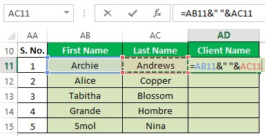
Hit ENTER & witness the magic!
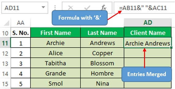
It is time that an old friend is paid a visit to get the remaining cells merged across the column – the Copy & Paste!
Copy the cell AD11 by right-clicking the cell & choosing the ‘Copy’ option or using the shortcut CRTL+C. The cell gets highlighted as shown below.
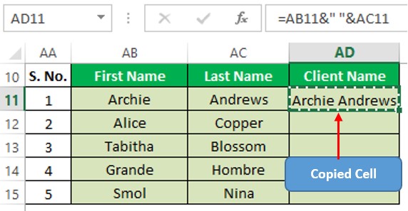
Select the remaining cells using the cursor or by holding the SHIFT + down arrow key (↓) from the cell AD12 as shown below.

Use the shortcut CTRL+V or right-click to choose ‘Paste’ for pasting the copied formula. Now the names within both cells in each row get merged into their corresponding cells in column AD.

Method 2 – The Concatenate Formula:
This method leverages one of the in-built formulae of MS Excel to merge the contents together. Before getting on with how to use put it into use, let us first understand its construction. Following is its syntax,
=CONCATENATE( text1, text2,……)
where, ‘text1, text2…‘ indicate the cells whose entries are to be merged together.
The very first step would be the inclusion of the equals sign (=) within the cell AD11 & type CONCATENATE followed by an opening parenthesis as shown below.

Once done click on the cell which needs to occupy the first portion of the merged entity which in this case would be AB11. Place a comma (,) following this selection & then include a space (“ “) before selecting AC11 – the cell containing the last name as shown below.
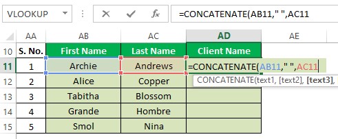
Close the parenthesis & hit ENTER.
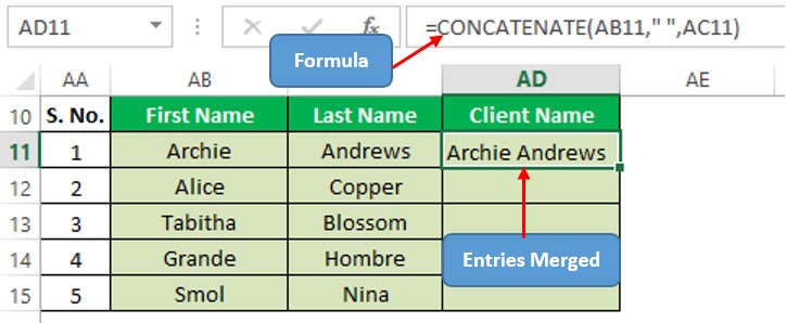
Copy this formula & paste it across the cells as shown in the previous method to get all the cells in both columns merged together.

Conclusion:
Hope this article was informative & helped you get a hold of merging 2 columns in MS Excel. Here’s one which elaborates on how to lock columns in MS Excel. There are numerous other articles too in QuickExcel that can come in handy for those who are in looking to level up their skills in MS Excel. Cheers!
