One may need to carry out basic mathematical calculations in Excel very often, to facilitate the process MS Excel provides inbuilt functions to deliver fast and accurate results.
Also read: Mathematical Functions in Excel – Part 1
Top Mathematical Functions in Excel
Here are few commonly used mathematical functions in Excel.
1. PI function
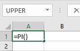
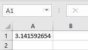
The Excel PI function calculates the value of the mathematical constant π up to 14 decimal places. In other words, the function returns 3.14159265358979. The PI function has the following syntax because it takes no arguments: PI(). Follow these steps to get the value of π in Excel:
- Select the cell where you want to display the result.
- Type =PI() in the formula bar.

- Press the Enter key to display the result.

2. PRODUCT function
The PRODUCT function in Excel calculates the product multiplication of a set of numerical values.
Syntax: PRODUCT(number1,number2,…), where number1, number2, etc. are the numbers for which you want the product or the cell references of the cells containing the numbers. The following example shows the use of PRODUCT function:
- Select the cell where you want to display the result.
- Type =PRODUCT(A1,B1,C1), where cells A1, B1, and C1 contain the first, second, and third numbers respectively.

- Press the Enter key to display the result.

3. CEILING.MATH function
The Excel CEILING.MATH function rounds a given number up to a specified multiple of significance. In general, positive numbers are rounded away from zero, while negative numbers are rounded towards zero. However, for negative numbers, the user can reverse the rounding way using the mode argument.
Syntax: CEILING.MATH(number, [significance], [mode]), where number is the number to be rounded, significance is the multiple to which it should be rounded and mode is a numeric parameter that only applies to negative integers and reverses the direction of rounding.
Negative integers are rounded towards zero if [mode] = 0 or is omitted and are rounded away from zero if [mode] = any other numeric value. The following example shows the use of CEILING.MATH function:
- Select the cell where you want to display the result.
- Type =CEILING.MATH(A1), where cell A1 contains the number. By default, significance is +1 for positive numbers and -1 for negative numbers.

- Press the Enter key to display the result.

4. FLOOR.MATH function
The Excel FLOOR.MATH function rounds a given number down to a specified multiple of significance. In general, positive numbers are rounded towards zero, while negative numbers are rounded away from zero. However, for negative numbers, the user can reverse the rounding way using the mode argument.
Syntax: FLOOR.MATH(number, [significance], [mode]), where number is the number to be rounded, significance is the multiple to which it should be rounded and mode is a numeric parameter that only applies to negative integers and reverses the direction of rounding. Negative integers are rounded away from zero if [mode] = 0 or is omitted and are rounded towards zero if [mode] = any other numeric value. The following example shows the use of FLOOR.MATH function:
- Select the cell where you want to display the result.
- Type =FLOOR.MATH(A1), where cell A1 contains the number. By default, significance is -1 for positive numbers and +1 for negative numbers.

- Press the Enter key to display the result.

5. EXP function
The EXP function in Excel determines the value of the mathematical constant e raised to a specified number’s power.
Syntax: EXP(number), where the number input is the real number you wish to raise e to. The following example shows the use of EXP function:
- Select the cell where you want to display the result.
- Type =EXP(2) in the formula bar to raise e to the power of 2.

- Press the Enter key to display the result.

6. LOG function
The Excel LOG function computes the logarithm of a given number in relation to a particular base.
Syntax: LOG(number, [base]), where number is the positive real number for which you want to compute the logarithm and base is an optional input that determines the base for calculating the logarithm. If the [base] option is missing, the default value of 10 is used i.e. the logarithm to the base 10 is calculated. The following example shows the use of LOG function:
- Select the cell where you want to display the result.
- Type =LOG(A1,4), where cell A1 contains the number and 4 is the base.

- Press the Enter key to display the result.

7. LN function
The LN function in Excel computes the natural logarithm of a given number.
Syntax: LN(number), where the number input is the positive real number whose natural logarithm you want to compute. The following example shows the use of LN function:
- Select the cell where you want to display the result.
- Type =LN(A1), where cell A1 contains the number.

- Press the Enter key to display the result.

Conclusion
In this article, we learned about some of the most commonly used mathematical functions in Excel.
References
