Spreadsheets are created bearing in mind that they would be accessed by a number of people, irrespective of whether it is going to be used in a school or college or any other organization for that matter. With too many people jumping on board it is of utmost importance to guard the credibility of the data that has previously been recorded.
Also read: How to Find Slope in MS Excel?
At times, some data as in the headers are never to be changed since they would be linked to data analysis tools such as Slicers or Pivot Tables.
So, this leaves us with no other option, than to restrict the access to those specific cells to safeguard their contents from being edited. In this article, we shall cover the stepwise procedure to lock the contents of a row & we shall be using the below tabulation to demonstrate that by locking the contents of its header row.

Locking a Row in MS Excel:
The first step is to select all the contents of the sheet by pressing CTRL+A and then to open the Font settings option by clicking on the button as shown in the below image.
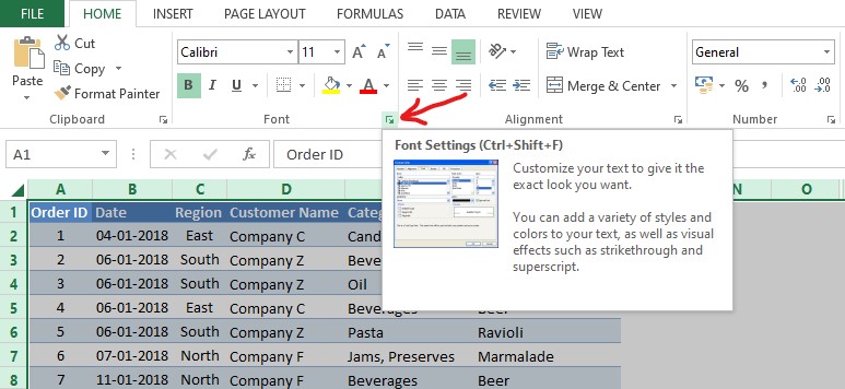
Those, who are fond of keyboard shortcuts might rather use CTRL+SHIFT+F to open the Font Settings. One has to be cautious while executing the shortcut & press the keys one after the other, rather than everything simultaneously. Once done, the Format Cells dialog box appears as shown below.
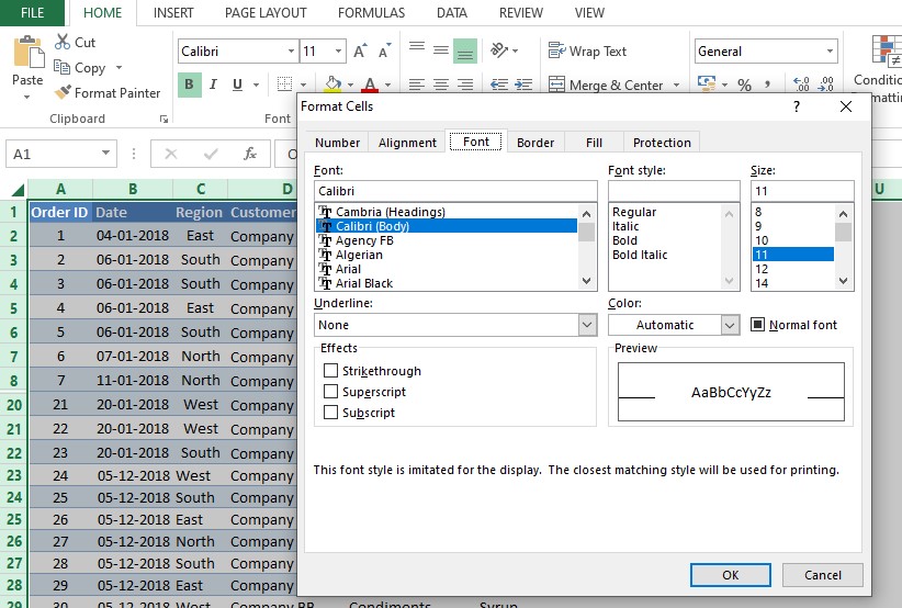
Choose the Protection Tab, in the above dialog box & uncheck the Locked checkbox, followed by clicking OK.
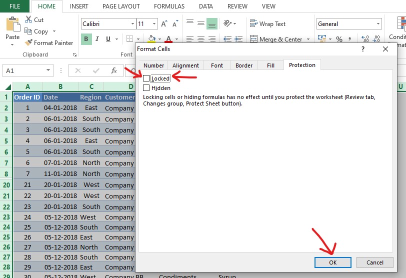
Now, the dialog box is gone & we are left to stare at the data tabulated.
What next, you ask? An important task!
It is here that we would be selecting the row that is to be locked.

Now the process is repeated again by opening the Format Cells dialog box. We again go to protection, but this time, the Locked checkbox is to be ticked!
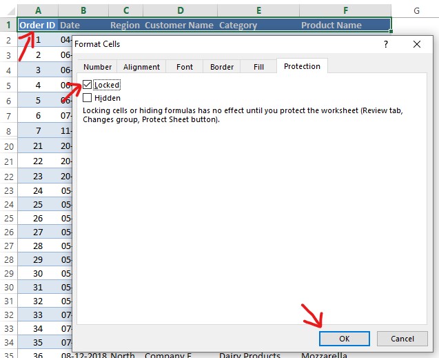
Now, if one thinks that clicking OK gets the job done – IT DOES NOT!
What has been done thus far, is to tell MS Excel which cells to protect when the sheet gets protected. Now, we move to the next part, where we protect the sheet. It is a fairly simple step, which needs us to go to the Review tab & locate the Protect Sheet option as shown in the below image.
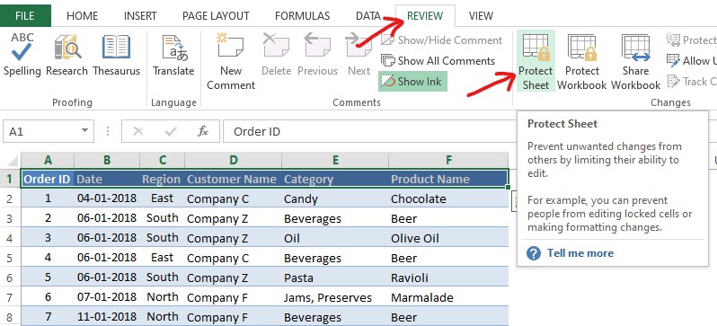
Click on the Protect Sheet option & a dialog box shall appear prompting to enter a password.
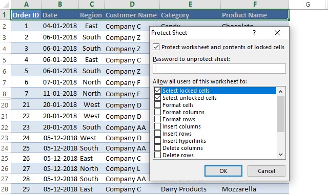
Type in a password of your choice & hit OK. There shall be another dialog box asking to confirm the password given earlier. Exercise this option with utmost care since there is no other way to unlock the protected row if the password given is forgotten.
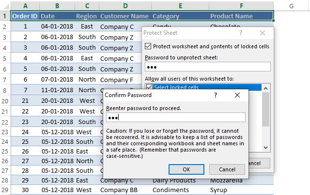
Hit OK & it’s all done now!
Try editing the contents of any cell in the header row & the following alert shall appear asking to unprotect the sheet before editing the cells.
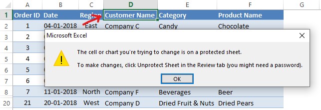
Great! But what if a situation arises that demands that the contents of the protected row be altered? What to do then?
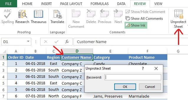
We might end up within the Review tab again, only to find that the Protect Sheet option has now been turned into Unprotect Sheet!
Click on that & a dialog box shall appear prompting for a password. The row becomes editable once the correct password is entered.
Conclusion
Hope the article was informative. QuickExcel has numerous other articles too which could help you with that one thing that you’re trying to do with MS Excel right now. Cheers!
