Some things are better left unsaid! This might be just true when it comes to the formulae used in MS Excel.
When you create a spreadsheet that pulls in values from various cells within a sheet or across different sheets to compute the intended results through formulae and put it around for circulation so that it gets updated by a group of people, then it is better to take all the measures within one’s power to make sure that these formulae are left untouched!
This article might just benefit those who have felt the need to do the aforementioned since it would be exploring ways to hide the formulae from being visible to the users.
Following is the dataset that shall be used throughout this article to demonstrate the process.
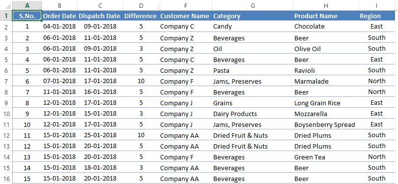
Reversing the Default Protection Settings of the Cells:
We shall get things started by selecting all the cells in the required worksheet in which the formula needs to be hidden using the keyboard shortcut CTRL+A.
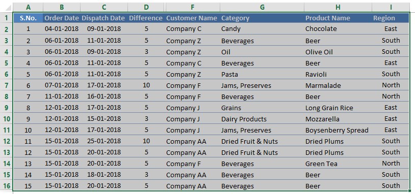
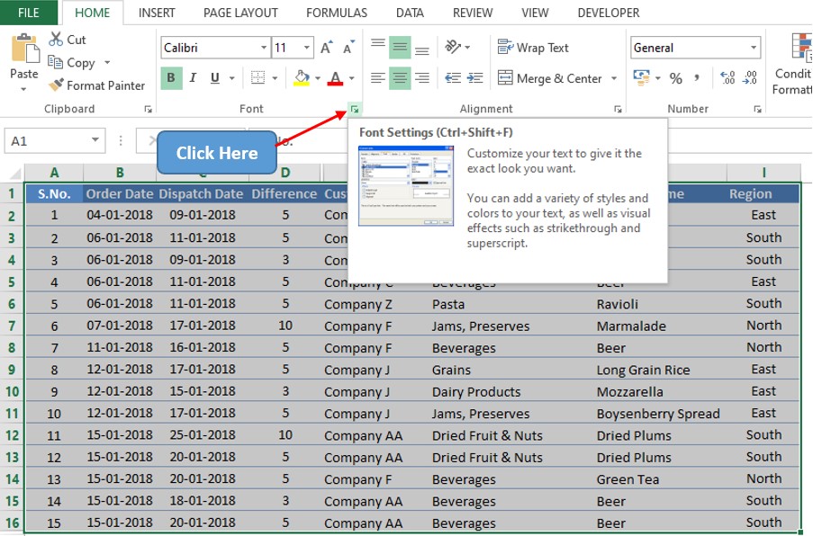
Once done, we shall now proceed to remove any default protection settings that might be applied to these cells by reaching out to the Format Cells pop-up.
This can be done by either using the keyboard shortcut CTRL+SHIFT+F or clicking on the ‘Extend’ button within the Font section of the Home tab as shown below.
This shall result in the following pop-up appearing. Navigate to the Protection tab of this pop-up as shown below.
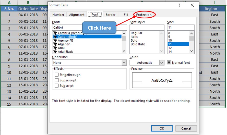
Once we are in the Protection tab, verify whether any of the checkboxes are already checked. If yes, we ought to uncheck those right away.
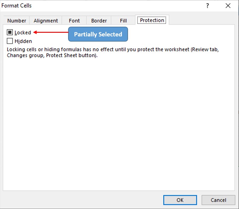
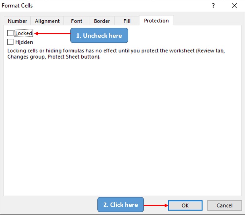
Upon clicking ‘OK’, the pop-up disappears.
Selecting All Cells with Formula:
Now, it is time to summon a built-in feature of MS Excel to select only the cells that contain the formula. This can be done by using the ‘Go To Special’ feature.
Use the keyboard shortcut CTRL+G & the following pop-up shall appear.
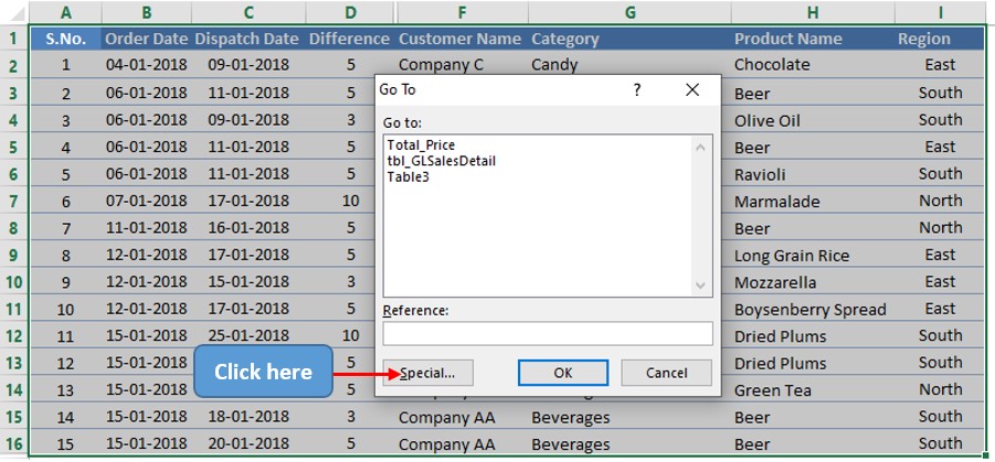
Clicking on the ‘Special’ option in the above image shall lead us to the following dialog box in which we ought to select the ‘Formulas’ option and keep the defaults as is so that it covers any formula within the selected range.
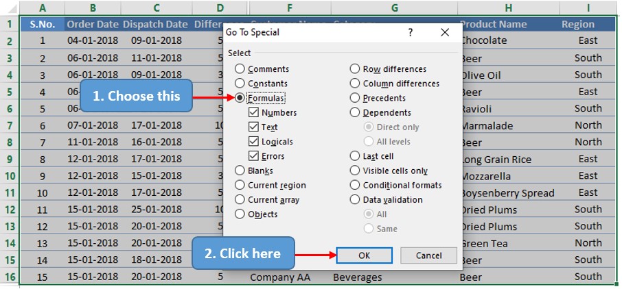
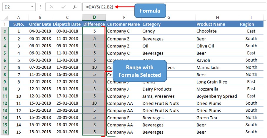
Once done, the selected range gets reduced to only the cells with the formula as shown below.
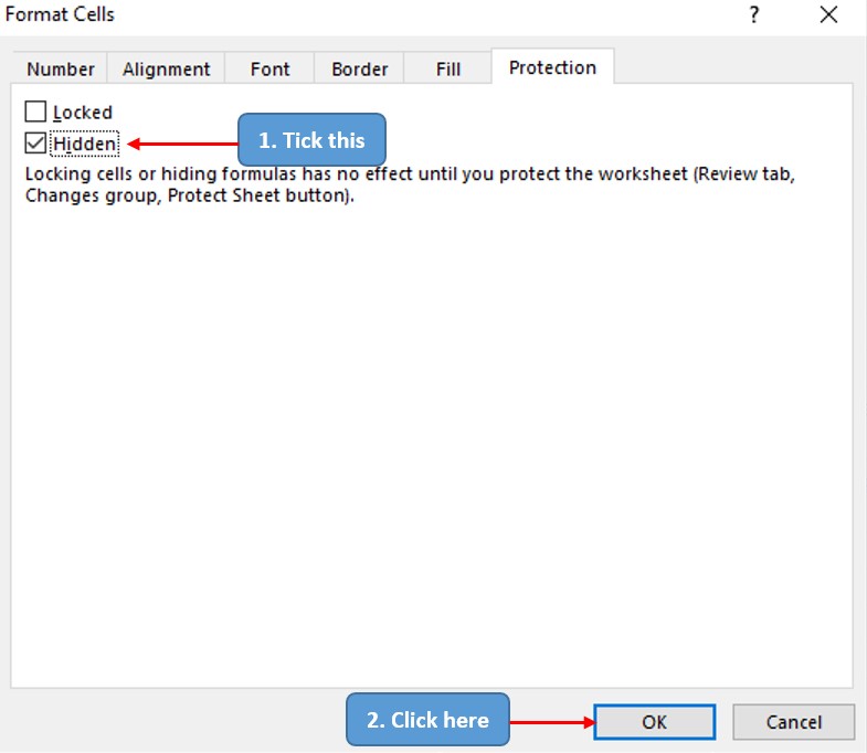
It is time we visit the Font Settings again by using either of the options stated earlier in this article. Now check the Hidden option within the Protection tab as shown below.
Once done, the pop-up waves goodbye & now we are left to stare at the screen.
Hiding the Formula:
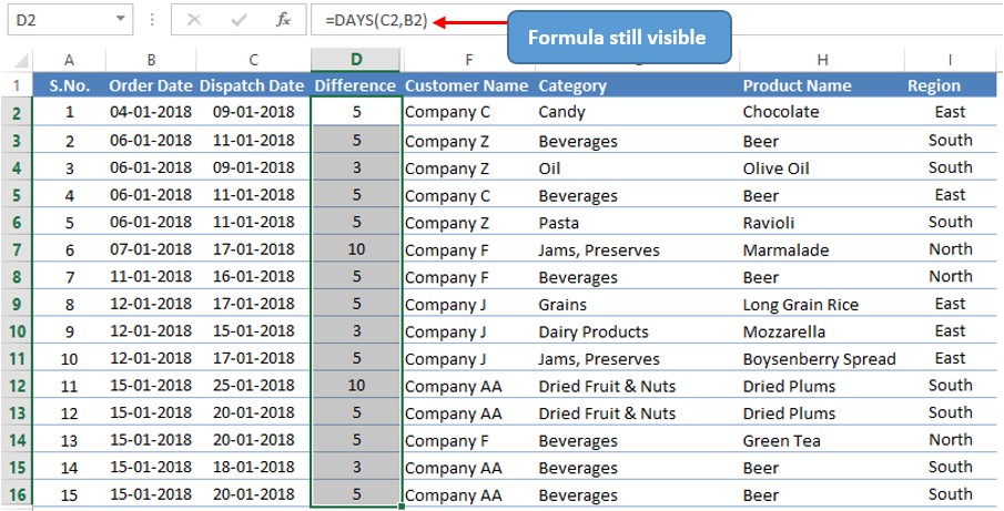
I can sense the reading wondering, ‘But hey! The formula is still visible.’ Yes, it is & we are going to make it vanish into thin air by navigating to the Review tab & select the Protect Sheet option as shown below.
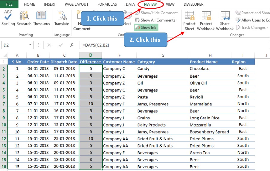
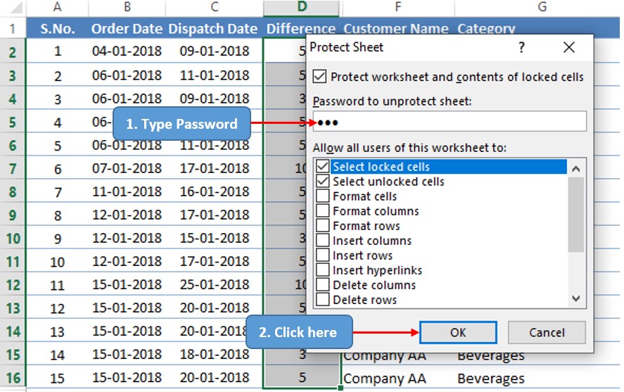
A Protect Sheet pop-up shall appear prompting for a password. Type in the password of your choice & click OK.
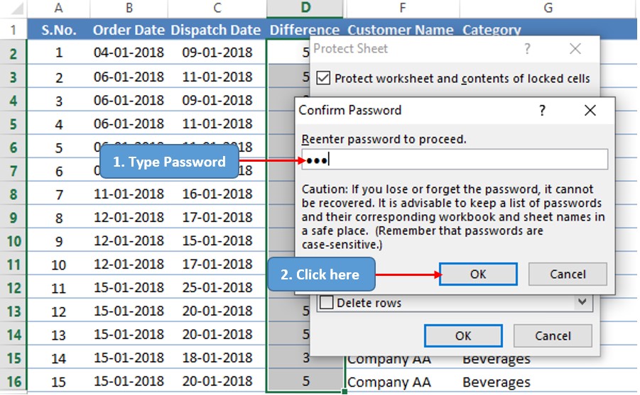
After clicking OK, MS Excel would want us to type the password again to confirm it. [Remember this password real good since there is no forget password feature in MS Excel.]
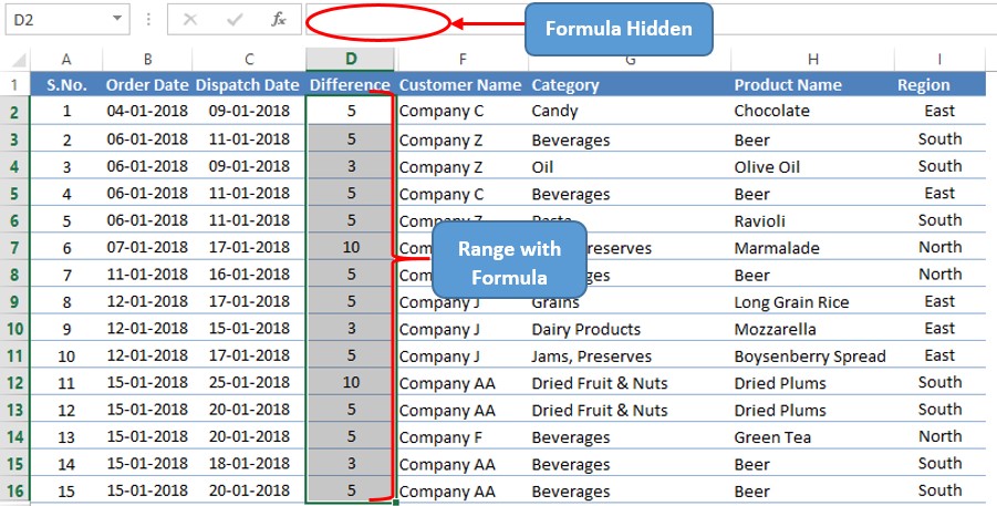
Hit OK & the formula within the selected range is no more visible!
Conclusion:
Now that we have got to the end of this article, hope it has given you what you came looking for. Here’s another one which elaborates on how to hide cells in MS Excel. There are numerous other articles too in QuickExcel that can come in handy for those who want to know more about MS Excel. Ciao!
