Let’s learn how we can find quartiles in Excel. A quartile is a statistical term that is used to describe the division of a dataset into four equal intervals. Each quartile has 25% of the total number of data points in a dataset. The four equal intervals are divided by three points namely – lower quartile, median and upper quartile. The median is the value that separates the upper and lower halves of a dataset or population or simply the middle number in a sorted list of numbers.
Find Quartiles in Excel Using the QUARTILE Function
The QUARTILE function in Excel returns the quartile of a data set. Syntax: QUARTILE(array,quart), where array is the numeric values or the cell ranges containing the numeric values and quart parameter specifies which value should be returned. When quart = 0, the minimum value of the dataset is returned, quart = 1 returns the first or lower quartile, quart = 2 returns the median value, quart = 3 returns the third or upper quartile, and quart = 4 returns the maximum value of the dataset.
Let us consider a sample dataset of numbers to be divided into quartiles:
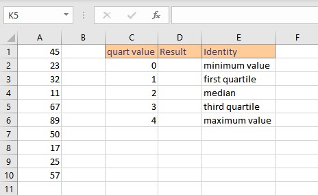
Finding the minimum value using the QUARTILE function:
- Go to cell D2 anf type =QUARTILE(A1:A10,0).
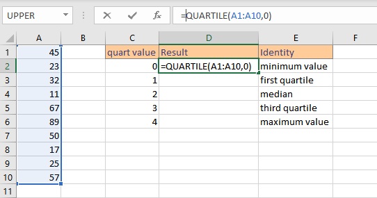
- Press the Enter key to display the result.
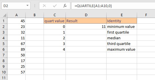
As you can see when quart = 0, the minimum value in the dataset = 11 is returned.
Finding the first or lower quartile using the QUARTILE function:
- Go to cell D3 and type =QUARTILE(A1:A10,1).
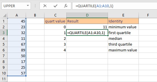
- Press the Enter key to display the result.

As you can see when quart = 1, the first or lower quartile of the dataset = 23.5 is returned.
Finding the median value using the QUARTILE function:
- Go to cell D4 and type =QUARTILE(A1:A10,2).
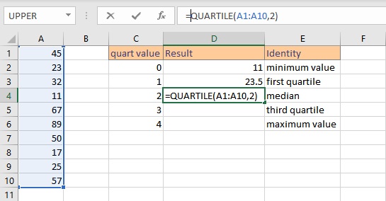
- Press the Enter key to display the result.
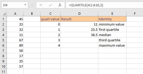
Here you can see that when quart = 2, the median value of the dataset = 38.5 is returned.
Finding the third or upper quartile using the QUARTILE function:
- Go to cell D5 and type =QUARTILE(A1:A10,3).
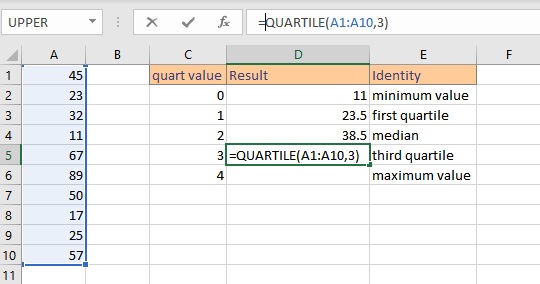
- Press the Enter key to display the result.
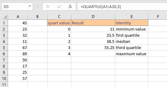
Here you can see that when quart = 3, the third or upper quartile of the dataset = 55.25 is returned.
Finding the maximum value using the QUARTILE function:
- Go to cell D6 and type =QUARTILE(A1:A10,4).
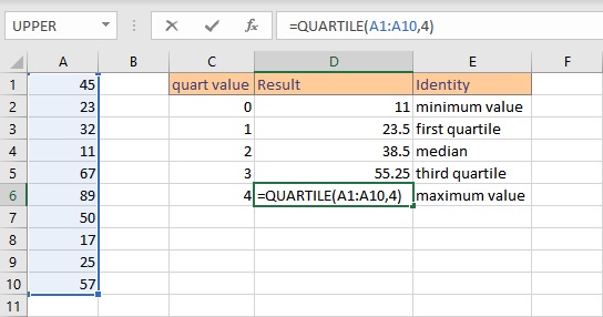
- Press the Enter key to display the result.
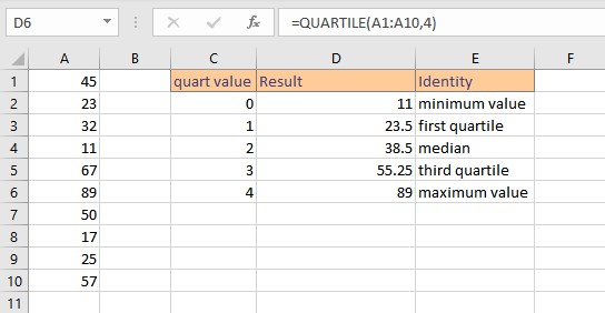
As you can see when quart = 4, the maximum value of the dataset = 89 is returned.
Note:
- The QUARTILE function returns the #NUM! error value if the array is empty.
- If the parameter quart is less than zero or greater than four, the QUARTILE function returns the #NUM! error value.
- If the parameter quart is non-numeric, the QUARTILE function returns the #VALUE! error value.
- The QUARTILE function returns the same value as MIN, MEDIAN, and MAX when the value of the parameter quart is 0, 2, and 4 respectively.
Highlight Quartiles in Excel
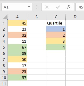
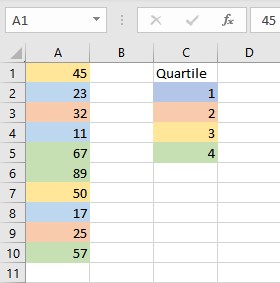
It is always good to highlight quartile values of a data set for easy identification. This can be achieved using Conditional Formatting in Excel.
First, select the color code for each quartile.
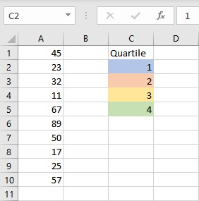
To highlight the data points above the third quartile:
- Select the cells containing the data points.
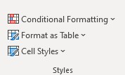
- Click on Conditional Formatting in the Styles group on the Home tab.

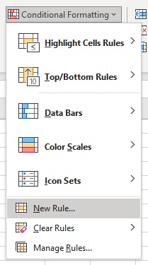
- From the drop-down that appears, click on New Rule… option.

- Select Use a formula to determine which cells to format option from the Select a Rule Type section in the New Formatting Rule dialog box.

- In the Format values where this formula is true text box, type =A1>=QUARTILE($A$1:$A$10,3) and select a color for highlighting as per the color code from the Format… option.
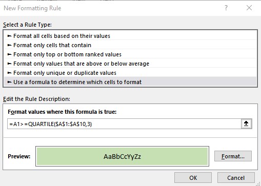
- Click in OK to complete the highlighting.
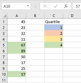
To highlight the data points in between median and third quartile:
- Select the cells containing the data points.
- Click on Conditional Formatting in the Styles group on the Home tab.

- From the drop-down that appears, click on New Rule… option.

- Select Use a formula to determine which cells to format option from the Select a Rule Type section in the New Formatting Rule dialog box.

- In the Format values where this formula is true text box, type =AND(A1>=QUARTILE($A$1:$A$10,2),A1<QUARTILE($A$1:$A$10,3)) and select a color for highlighting as per the color code from the Format… option.
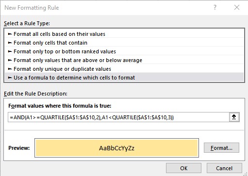
- Click in OK to complete the highlighting.
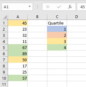
To highlight the data points in between the first quartile and median:
- Select the cells containing the data points.
- Click on Conditional Formatting in the Styles group on the Home tab.

- From the drop-down that appears, click on New Rule… option.

- Select Use a formula to determine which cells to format option from the Select a Rule Type section in the New Formatting Rule dialog box.

- In the Format values where this formula is true text box, type =AND(A1>=QUARTILE($A$1:$A$10,1),A1<QUARTILE($A$1:$A$10,2)) and select a color for highlighting as per the color code from the Format… option.
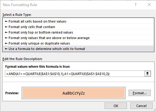
- Click in OK to complete the highlighting.
To highlight the data points in below first quartile:
- Select the cells containing the data points.
- Click on Conditional Formatting in the Styles group on the Home tab.
- From the drop-down that appears, click on New Rule… option.
- Select Use a formula to determine which cells to format option from the Select a Rule Type section in the New Formatting Rule dialog box.
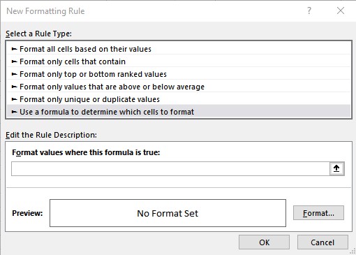
- In the Format values where this formula is true text box, type =AND(A1>=QUARTILE($A$1:$A$10,0),A1<QUARTILE($A$1:$A$10,1)) and select a color for highlighting as per the color code from the Format… option.
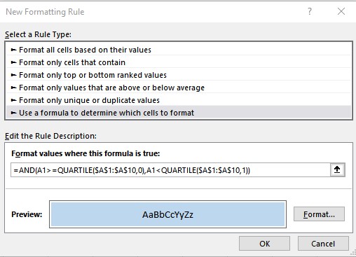
- Click in OK to complete the highlighting.
Conclusion
In this tutorial, we learned how to find quartiles using an inbuilt function QUARTILE and to highlight them using Conditional Formatting for easy identification in Excel.
