We all have a spreadsheet filled with data and would eventually end up analyzing them. As an essential pre-requisite, we would be selecting the desired data to get started. But, what if we select more than what is required or what if we need to leave a specific portion of cells while selecting a row or a column?
Absolutely not! It is not required to start from scratch again by carefully selecting each of the desired cells. Rather, there seems to be a way around to do the converse of selecting in MS Excel – Deselecting!
We are going to elaborate just that in this article.
It is always advisable to get familiarized with more than one technique. So, we are going to cover a couple of techniques each serving its own purpose.
- Deselecting Specific Cells
- Deselecting in Mass Selection
Deselecting Specific Cells
In the following table, let’s say we need to select all the contents except for those in rows 6 & 7 for instance.
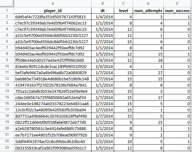
Seems a bit weird right?
It wouldn’t be by the end of this section.
By the conventional practice, we would click cell A1 to select it & drag the mouse all the way down to row 23 as shown below.
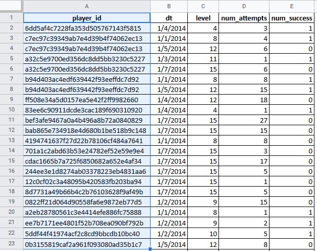
Without lifting that finger off the left mouse button, drag it onto the subsequent columns till it reaches cell E23.
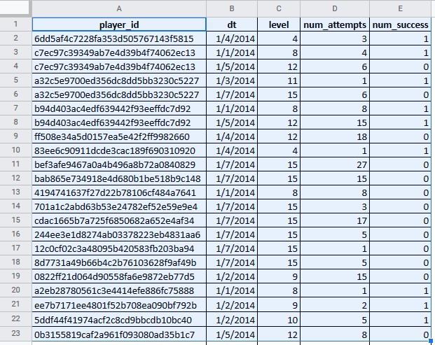
Before we can call it done & dusted, we need to remove rows 6 & 7 from the selection.
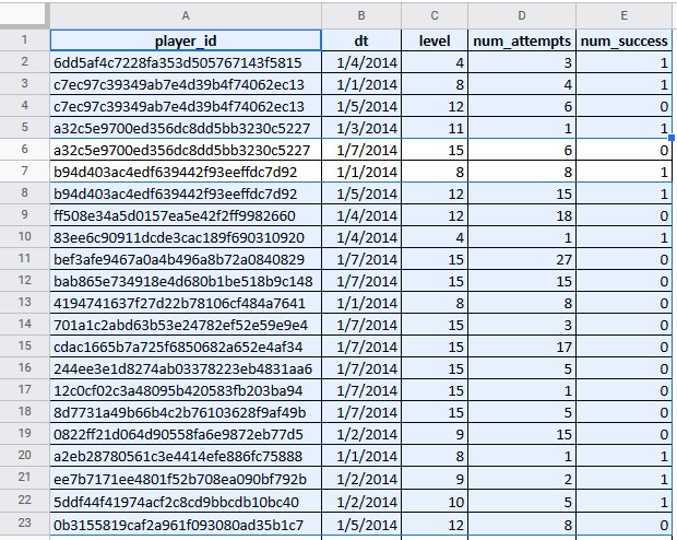
This can be done by pressing the CTRL key and then selecting the required parts by clicking & dragging using the left mouse button (the same way that we use for selecting the cells).
Once done, the selected parts are removed from the selected portion as given in the below image.
Deselecting in Mass Selection
Selecting the contents can really be tough when there is a humongous amount of data spreading through hundreds of rows. While if this is the case of selecting the contents, need I emphasize how hard would it be to deselect?
Let us consider the following table which has a vast expanse of data.
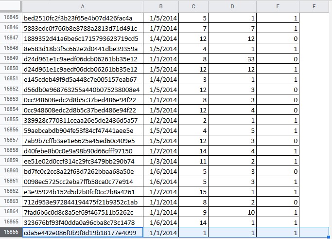
Selecting the contents in a tabulation of 16,866 rows is no big deal. As a common practice, we’d start by clicking on the very first cell which we would like to include in the selection, and drag the mouse from thereon.
Having done that let’s say we have selected the entire contents of the tabulation as shown below.
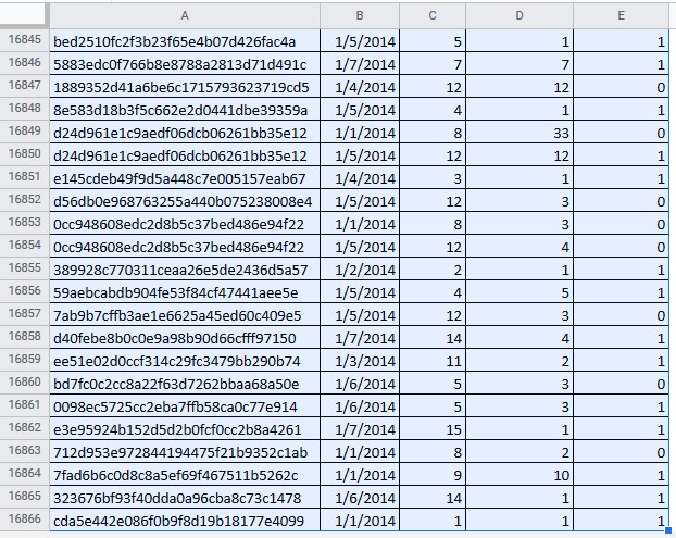
But now out of nowhere, just after that finger pressing over the left mouse button is raised, we are hit with the thought that the contents of only the first three columns alone are needed. Tough luck, eh?
Worry not! The SHIFT and the arrow keys come to the rescue.
Press the SHIFT key first & then hit the left arrow key (←) to deselect the entire column E. The key here is to press the SHIFT & the left arrow key one after the other & NOT SIMULTANEOUSLY.
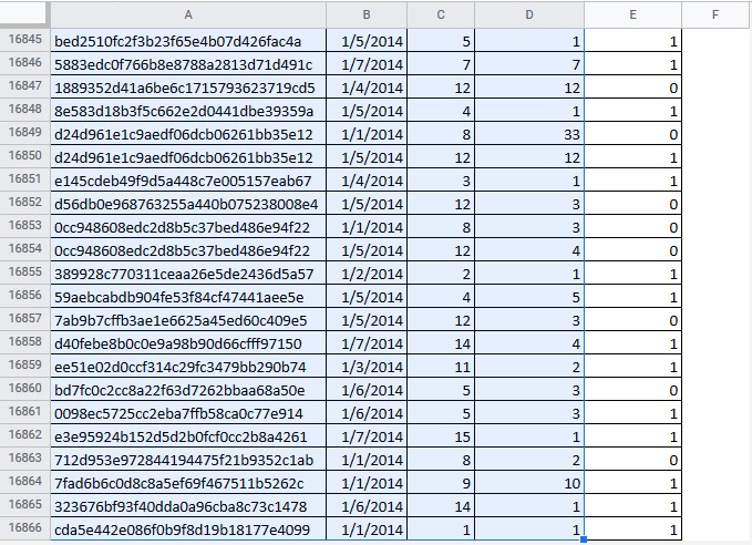
Similarly, the same approach can also be used to deselect the contents in whatever directions necessary by pressing on the appropriate arrow key.
Conclusion
So, here we are, having covered two different techniques to deselect contents in MS Excel. Sure that this would save much time by reducing the number of start overs while selecting the data. The word on the web is that Microsoft has made this feature available only for the versions released after Office 2019. Should you have something lesser, it’s time to reconsider.
Do watch out QuickExcel to keep yourself abreast with the updates & nuances of MS Excel. Cheers!
