Data is always not refined. This is the one thing that would always give migraines to those who work with tonnes of data. Getting down to those which really matter can be quite tedious & this article is going to suggest ways to tackle one such situation. In this article, we will explore the steps in which one can count the unique values in any given tabulation of data using MS Excel.
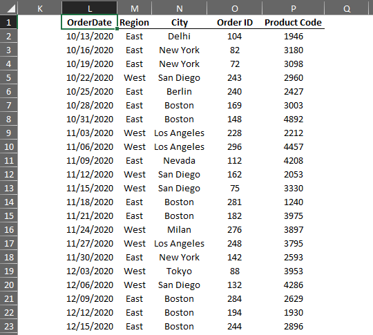
Let us consider the above data in which the names of the cities tend to get repeated. Should one desire to know the count of cities in this list, then the path to results is as follows.
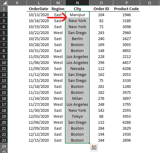
Select all the entries of column N which contains the name of the cities as shown below.
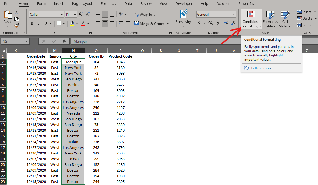
Then move the cursor towards the Styles section of the Home tab where one can find the Conditional Formatting as indicated in the below image.
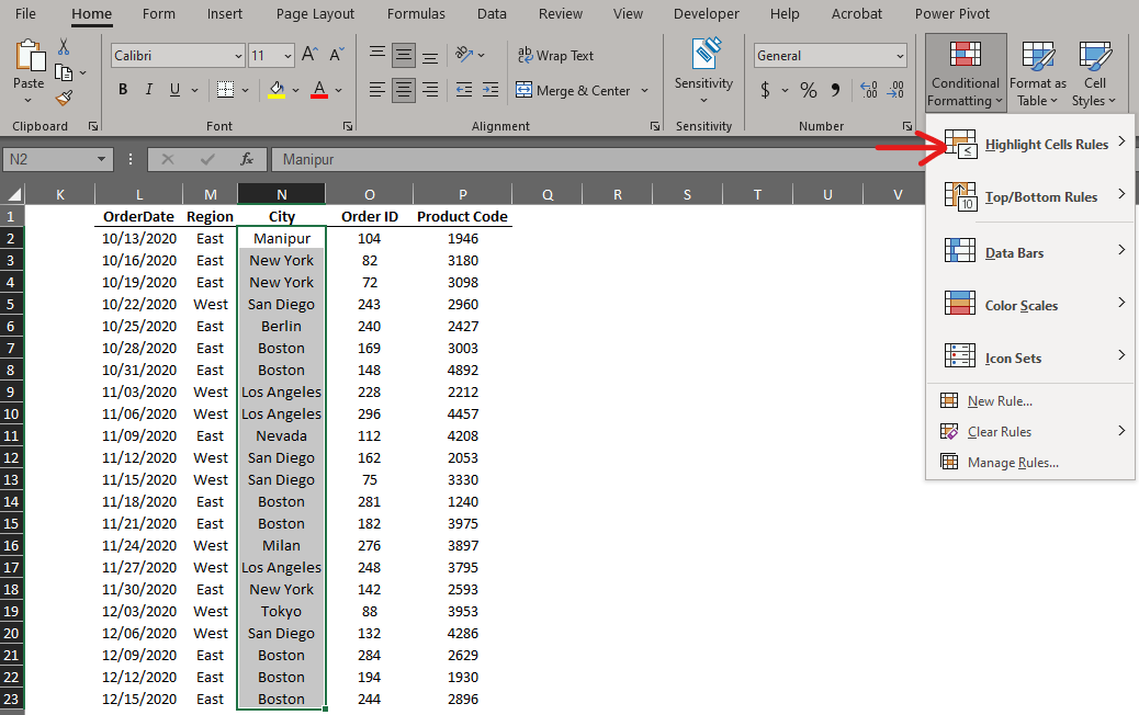
Then click on Conditional Formatting which would list a series of options from which one needs to choose the Highlight Cells Rules as shown below.
Once done, another list shall appear from which one needs to choose the Duplicate Values option as shown in the below image.
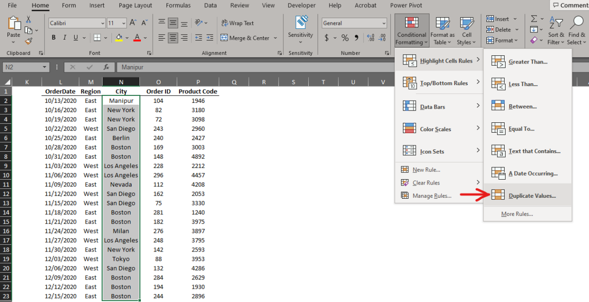
Now there would be visible changes in the cell colours within the selected range & also a pop-up prompting to choose the desired colour to highlight the duplicate values.
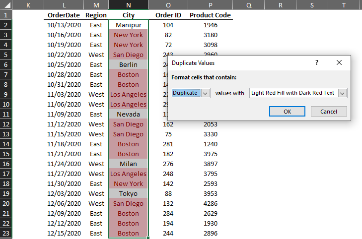
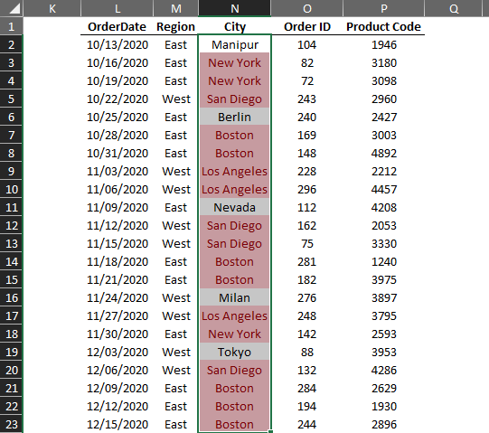
In this example, we are going to stick to the default selection of light red fill with dark red text & click OK. The pop-up is now gone leaving us to stare at the data highlighted with duplicates.
Now one shall proceed with selecting the header row of the data & apply the filter by clicking on the option with the very same name as indicated below.
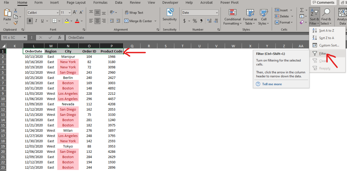
Those who are used to keyboard shortcuts may use the CTRL+SHIFT+L to apply the filter. The keys are to be pressed one after the other without lifting the finger off the preceding key in the same sequence as stated above. After the filter is applied click on the dropdown in the column titled City.
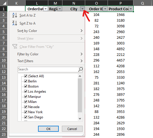
Select No Fill within Filter by Color as shown in the below image.
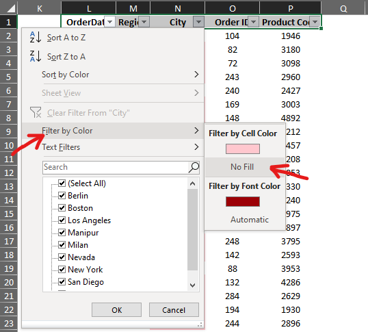
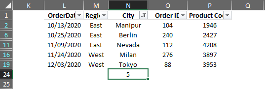
Now the data will be filtered displaying only the cells without any fill, which means that now we are eye to eye with the unique values as depicted in the image below.

Now click on the cell below the last entry of column N which in this case would be below Tokyo. A formula shall now be constructed with an equals sign (=) followed by SUBTOTAL and an open parentheses as shown below.
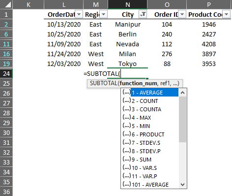
Select 3 for COUNTA which counts the number of non-blank cells in the selected range & then select the range of filtered cells in column N.
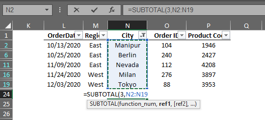
Include the closing parentheses & hit ENTER. Now the total number of unique values in the selected range shall be displayed!
Summary
Now we have reached the end of this article detailing how to count unique values in MS Excel. Hope it brought to you what you were looking for. But what if you want to know about removing the duplicate values in MS Excel? Go on & read this article which elaborates on the necessary details. QuickExcel has numerous other articles too that can come in handy for those who are in a quest to know something more in MS Excel. Cheers!
