Everything we humans look into, we shall name. It’s near impossible for us to comprehend something without tagging a name to it. There has got to be a name for everything!
It has been that way since time immemorial & it will be the same years into the future. How are we even going to say about something if there ain’t a name to it?
The same goes for the charts that we create in MS Excel too. There may be a chunk load of data which would be analysed for comparison against each other in charts, but how does one get around differentiating them from one another?
Yes, there are different colours that would do the purpose, but going back to the very start of the article – where are their NAMES?
That is exactly what we are going to explore in this article. We shall use the below chart to demonstrate the editing of Series Name. Let us get started!
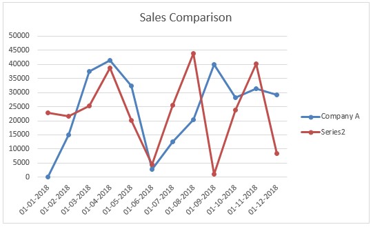
Editing Series Name
With closer observation, one can find that the blue line has been identified as ‘Company A’ whilst the red line has been identified as ‘Series 2’! Sounds a bit weird right? It makes no sense in comparing the sales of ‘Company A’ with something as vague as ‘Series 2’.
Should someone opine that ‘Series 2’ is the name of a company, please be informed that it is the default naming that MS Excel comes up with for data series in a chart. The objective here is to change ‘Series 2’ into ‘Company B’.
With a helping hand from the mouse, we resort to the oldest trick in the book – the Right Click!
Move the cursor towards the chart area & right click anywhere within the chart area. Once done, the following menu with an extensive list of options to choose from appears.
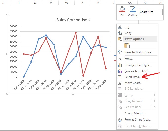
Choose the Select Data option from the list as indicated in the image above & the following pop-up shall appear.
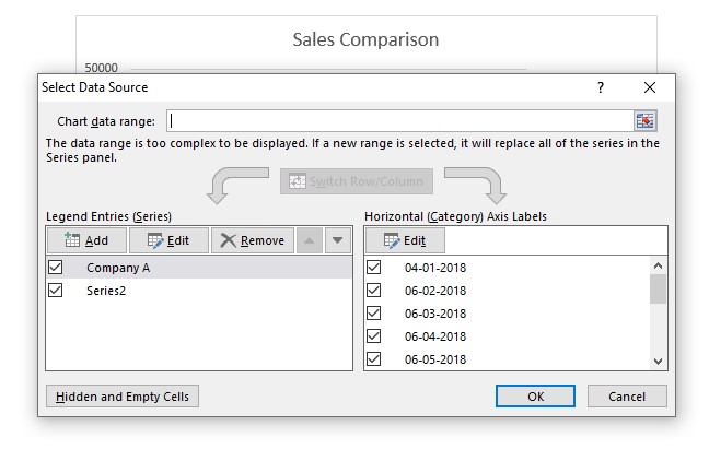
Select the ‘Series 2’ under the Legend Entries section & then click on the Edit option located right above in the middle as shown below.
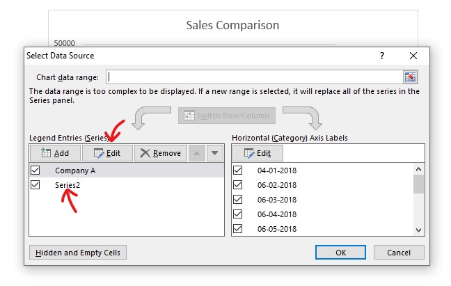
Once done, it shall take you to another pop-up – the Edit Series pop-up, which is the one we have been looking for ever since to get the job done. It’s time that we specify the name of the series as ‘Company B’ within the Series name text box indicated in the image below.
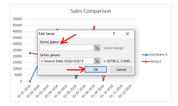
The moment one clicks the OK button, the names of the series displayed change from the earlier shown ‘Series 2’ to ‘Company B’ in no time. The same would also be reflected in the Select Data Source pop-up which reappears after the Edit Series pop-up goes out of sight.
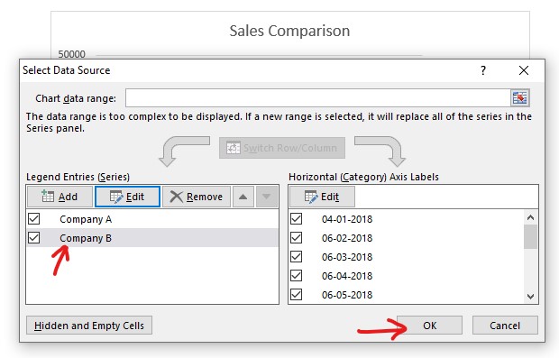
Click OK & the Select Data Source pop-up disappears, only to put the chart with the updated series name within our sight.
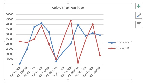
And that is the sequence of tasks that one should know to carry out the modification of a series name not only in line charts but also for the other formats of the chart as well.
Summary
Now that we have reached the end of this article detailing how to change Series Name in MS Excel, hope it has provided you with sufficient information. Here is something that elaborates on How to Edit Legends in MS Excel?. If you are someone looking for sources to enrich your know-how in MS Excel, then QuickExcel is the place to be & the list of articles available would lay a concrete foundation for you to achieve this feat. Ciao!
