Circular references in Excel are formulas that, in their chain of calculations, access their own or another cell several times, resulting in an unending loop that greatly slows down your spreadsheet.
In Excel, a circular reference means that the computation in a specific cell refers to its output once or multiple times.
Also read: How to Calculate Standard Deviation in Excel?
Why Should We Avoid Circular References in Excel?
When you have a huge spreadsheet containing hundreds of formulas and data values, circular references in Excel pose a significant risk of miscalculation and misinterpretation.
Other difficulties include Excel returning zero when you move to formula editing form by mistake either by double-clicking or clicking F2, without making major changes to the formula and then tapping the enter key. If you don’t want to run into any problems, prevent using circular references in Excel.
Find Circular References in Excel
Let’s start from the basics. In Excel, a circular reference happens when a formula refers to its own cell directly or indirectly.
There are two types of Circular References:
- Direct Circular Reference – When a formula in Excel refers to its own cell, it is known as a direct circular reference.
- Indirect Circular Reference – When a formula in Excel, indirectly refers to its own cell, this is known as an indirect circular reference.
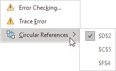
For Example, there are two circular references on our Excel sheet. There is one direct circular reference (A3) and one indirect circular reference (A4) (D2, C5, and F4).

- In your Excel worksheet, click the down arrow beside Error Checking and select Cell References from the Formula Auditing group to discover circular references.
To find all Circular References:
- Go to Formulas in the Home tab.
- Click on Error Checking from the Formula Auditing group on the Formulas tab to reveal a drop-down menu.
- Select Circular References from the function menu. One circular reference’s cell address is displayed already

- You can also use the status bar to see the status of any circular references, status shown at the bottom of the Excel worksheet.
- Now, fix the circular reference (this article does not cover fixing of circular references)
- The final result, of our sample data, after fixing of circular reference:

- Continue these steps to identify other Circular References in your worksheet. Now, Tap the down arrow next to Error Checking in the Formula Auditing group on the Formulas tab.
- Again, Select Circular References. The indirect circular reference cell addresses are shown in Excel.

Example of a Circular Reference
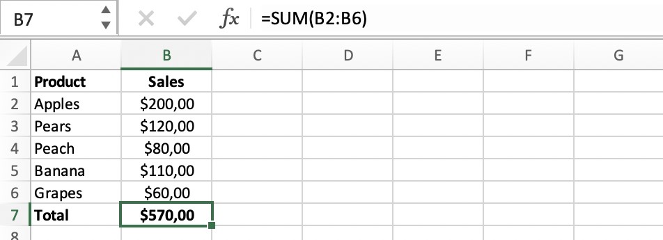
Suppose, the total of fruit sales of a Grocer is calculated in cell B7 in the sample below i.e., sum of cell ranges B2:B6. There is nothing incorrect about the following calculation:

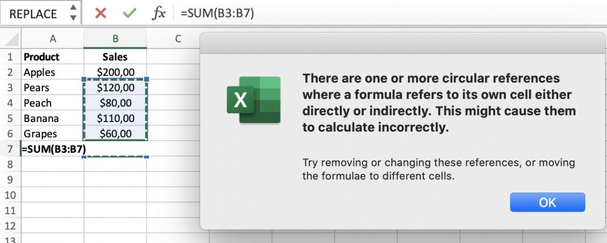
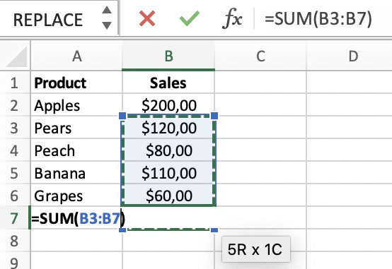
- If we use B3:B7 rather than just B2:B6, the function in cell B7 will do a calculation that contains the outcome of this precise calculation:

- Of course, this isn’t conceivable. One or more circular references are detected by Excel.
- The value ‘0’ is printed as error in cell B7 after tapping ‘OK’ in the notification show up:

Conclusion
That’s It! Hope you have learned about circular references in Excel and now you can now easily find circular references in your Excel worksheet.
We hope you learned and enjoyed this lesson and we’ll be back soon with another awesome Excel tutorial!
