This tutorial is an easy step-by-step guide to calculating frequencies, ratios, and percentages in Microsoft Excel. We will learn to calculate these elements with the help of formulas, appropriate examples, and supportive images.
Steps to calculate frequency in Excel
We will take a sample mark list of students that contains the grades and percentage of marks. We want to find out the frequency of each grade in the mark list.
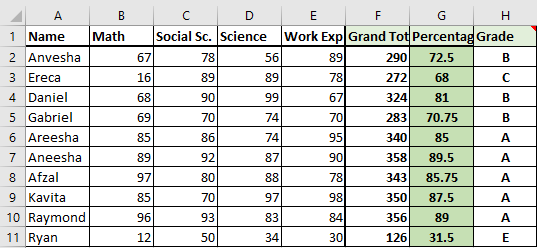
To calculate frequency in Excel, follow these steps.
- Create a table with the following headings- Grade, Percentage, Interval, and Frequency.
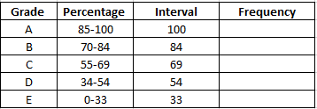
- Under Grade, list down all the grades such as A, B, C, etc.
- Under Percentage, make a class interval of the percentage marks for highest to lowest marks. For example- 95-100, 85-94, 75-84, etc.
- Under Interval, list down the lower limits of all class intervals. For example- 100, 94, 84, etc.
- Under Frequency, apply the FREQUENCY formula.
- Type =FREQUENCY( and select the percentage range in the mark list for the argument named data_array.
- Put a comma and select the interval column range for the argument bins_array.
- Close brackets and hit ENTER.
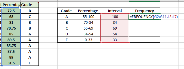
You can see that the cell now displays the frequency of A grade in the mark list.
- Drag the cell down from the lower right corner till the bottom to autofill the FREQUENCY formula to the entire column.
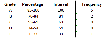
You can see that the formula has been applied to the entire column displaying frequencies of all grades.
Steps to calculate the ratio in Excel
There is no particular formula to find ratios in Excel. We must first calculate the GCD or greatest common divisor of the two numbers and then find out the ratio from it.
To calculate GCD, follow these steps.

- Type the two numbers for which you want to find the GCD in two different cells.
- In the blank cell, type the GCD formula. This is how the GCD formula syntax looks like.
=GCD(number1, [number2],…)
- Select the first number for argument number1.
- Select the second number for the second argument [number2].
- Close brackets and press ENTER.
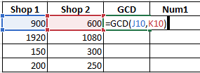
- Drag the cell down from the lower right corner to autofill the GCD formula in the cells below.
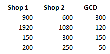
You can see that we have successfully found the GCD for all other numbers in the table.
- Now, in the Num1 and Num2 columns, divide each number with their GCD as done in the images below.


- Drag the cells down to get the ratio elements for the entire column.

We must now join the two elements of a ratio together in a cell and depict them in the ratio format. Follow these steps.
- In a cell under the Ratio column, type = and select the first number from the Num1 column.
- Put the & (ampersand) sign.
- Put a : (colon) between two double-quotes like this “:”
- Put the & again and select the second number from the Num2 column.
- Press ENTER to get the ratio format.
This is how the values in the cell should look like before you press ENTER.

We have now found the ratios for the entire column.

Steps to find percentage in Excel
Finding percentages is a very easy task in Excel. We will learn the easiest way to find the percentage of a number with the help of the steps below.
We take an example of a mark list again to find the percentage of the grand total marks of the students.
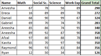
To find the percentage of the total marks, follow these steps.
Recommended read: How to Use SUM functions in Excel?
- First, find the sum of marks scored in each subject using the SUM function.
- Type =SUM( and select marks scored for all the subjects.
- Close brackets and press ENTER.

- Drag the cell below to autofill the SUM function.
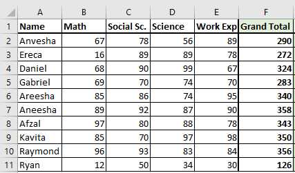
- Create a new column named Percentage in the same table.
- Type = and select the first number in the Grand Totals column.
- Divide the grand total with the total marks of all subjects. For example, we have 4 subjects with 100 marks in total, so the total of all subjects will be 400.
- Now, put an * (asterisk) and type 100. This means we are now multiplying by 100.
- Press ENTER to get the percentage.
This is how the formula must look like before pressing ENTER.

- Drag the cell below to get the percentage of all the students.
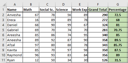
You can see that the percentage marks are displayed for all the students.
Conclusion
This was all about the detailed steps to calculating frequency, ratio, and percentage in Microsoft Excel. Stay tuned for more informative tutorials like this.
Reference- Contextures
