In Excel, P-Values are also known as probability values, and they are used to determine the statistical significance of a finding. The P-Value is used to determine whether the Null Hypothesis is valid.
If the null hypothesis is deemed implausible by the P-Value, we might conclude that the alternative hypothesis is likely to be correct. Essentially, it allows us to determine whether the presented results are due to chance or show that we are evaluating two unrelated topics. As a result, P-Value is a detective rather than a judge.
Formula for P-Value
A P-Value is a number between 0 and 1, although it’s better to think of them as percentages (for example, a P-value of 0.05 equals 5%). The null hypothesis is rejected when the P-Value is low.
Finding the P-Value for correlation in Excel is a reasonably simple process, but there is no single function for the task; we’ll look at an example.
Formula to calculate P-value:
=TDIST(x, deg freedom, tails)
Null Hypothesis
The null hypothesis is the idea that there is no relationship between two things when we compare them.
Before we can compare two objects, we must first establish that there is some sort of relationship between them.
When a P-Value rejects the null hypothesis, we can state that both of the things we’re comparing have a good likelihood of being true.
Methods To Calculate P-value In Excel
Let’s understand the P-value by using some examples.
Method 1: Using Step-by-Step calculation
In this example, we’ll use Excel to determine the P-Value for the given data.
- We have gathered data of various cricketers, against the runs players have scored in a given series.
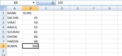
- We’ll need another tail for this; we’ll need to know how many runs each batsman is projected to score.
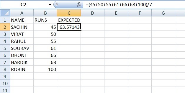
- By dividing our sum of counts by the number of runs, we can obtain the average runs for every player in the expected runs column.
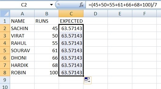
- By dividing our sum of counts by the number of runs, we’ve discovered the predicted value. It’s roughly average, while ours is 63.57.
- As can be seen from the data, we added the estimated runs column by placing the formula in cell C3.
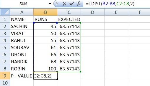
- To get the P-Value for this expression, use the formula TDIST(x, deg freedom, tails).
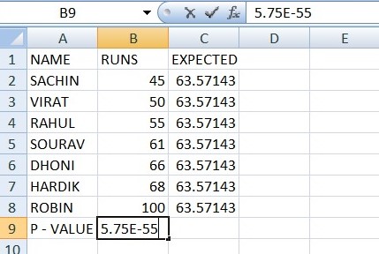
As a result,
- x denotes the range of our data, which is divided into runs.
- deg freedom = the range of our expected values’ data.
We want the solution for two tails, therefore tails = 2.
- We can observe that the outcomes we obtained are nearly zero.
- As a result, we can conclude that the null hypothesis is supported by substantial evidence in this case.
Method 2: Using Formula
- For the time being, let’s assume some values to determine the evidence’s support.
- For our formula =TDIST(x, deg_freedom, tails).
- If we use x=t (test statistics), deg freedom = n, and tail = 1 or 2, we get the following results.
- As we’re seeing, the results are 27.2 percent if we look at them in percentages.
- When the values of x, n, and tails are provided, you may use this method to find the P-Values.

Conclusion
That’s It!. We hope you have learned what is P-value in Excel and how to calculate P-value in Excel. We’ll be back soon with another awesome Excel tutorial!
