Lookup and Reference Functions in Excel

Lookup and Reference functions help you work with data arrays and come in handy when you need to work across multiple data sets. They can provide information about a range, retrieve the location of a given address or value, or seek up specific values. Here are some of the lookup and reference functions.

Lookup and Reference Functions

Let’s get started with the last part of our lookup and reference functions series. If you haven’t read through the last 3 parts, here are the links to the same:

1. UNIQUE function

The UNIQUE function in Excel returns a list of unique values inside a list or range. Text, numbers, dates, and times, among other things, can be used as values.

Syntax: =UNIQUE(array,[by_col],[exactly_once]), where array is the Range containing unique values, by_col is optional: FALSE (default) for by row search, TRUE for by column search and exactly_once is optional: TRUE for values that occur only once and FALSE for all unique values (default).

The following example shows the use of the UNIQUE function:

Select the cell where you want to display the result.
Type =UNIQUE(A1:A10,FALSE,TRUE), where cells A1:A10 contain a list of colours.

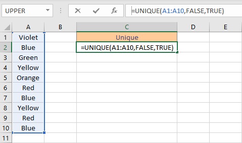
Press the Enter key to display the result. It returns the name of colours that occur only once in the range.

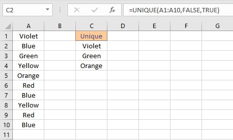
Note: This function is available only in Office 365.

2. VLOOKUP function

VLOOKUP is an Excel function that searches for data in a vertically structured table. It allows both approximate and accurate matching, as well as wildcards (*?) for partial matches. The function expects lookup values to be in the first column of the table provided to it.

Syntax: VLOOKUP (lookup_value, table_array, col_index_num, [range_lookup]), where lookup_value is the value to look for, table_array is the table to look up for a value, col_index is the column number to retrieve data from, and range_lookup is a boolean value that indicates whether a match is exact or approximate. The default value is TRUE indicating an approximate match.

The following example shows the use of VLOOKUP function:

Select the cell where you want to display the result.
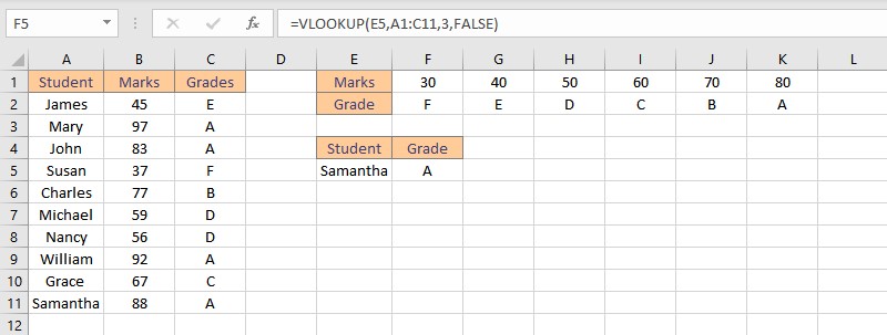
Type =VLOOKUP(E5,A1:C11,3,FALSE), where E5 contains the lookup value, cells A1:C11 contain the table to lookup, data is retrieved from column 3 of the table, and FALSE for an exact match.

Press the Enter key to look up for and display the grade obtained by Samantha.

Note: Use the new XLOOKUP function, which is a better version of VLOOKUP that works in either direction and provides precise matches by default, making it easier to use than its predecessor.

3. XLOOKUP function

The Excel XLOOKUP function replaces earlier functions like VLOOKUP, HLOOKUP, and LOOKUP with a more modern and flexible version. Approximate and exact matching, wildcards (*?) for partial matches, and lookups in vertical and horizontal ranges are all supported by XLOOKUP.

Syntax: XLOOKUP(lookup_value, lookup_array, return_array, [if_not_found], [match_mode], [search_mode]), where:

lookup_value is the value to look for
lookup_array is the range to look up a value for
return_array is the array or range to be returned
not_found is optional the value to be returned if no match is found
match_mode is optional: 0 for exact match (default) -1 for exact match or next smallest, 1 for exact match or next larger 2 for wildcard match
search_mode is optional:
1 for search from first (default), -1 for search from last, 2 for binary search ascending, and -2 = binary search descending.

The following example shows the use of XLOOKUP function:

Select the cell where you want to display the result.
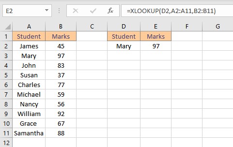
Type =XLOOKUP(D2,A2:A11,B2:B11), where D2 contains the lookup value, cells A2:A11 contain the list of names to search from, and cells B2:B11 contain the list of marks to return the result.

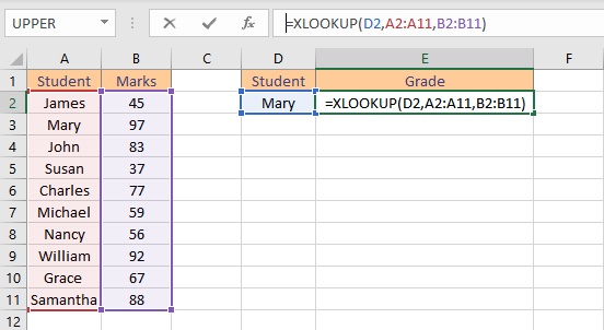
Press the Enter key to display the result. It returns the marks obtained by a student named “Mary”.

Note: This function is available only in Office 365.

4. XMATCH function

The XMATCH function in Excel conducts a lookup and returns a value in either vertical or horizontal ranges. It is the MATCH function’s more robust and flexible replacement. Approximate and exact matching, reverse search, and wildcards (*?) for partial matches are all supported by XMATCH.

Syntax: XMATCH(lookup_value, lookup_array, [match_mode], [search_mode]) , where lookup_value is the value to look for, lookup_array is the range to look up a value for, match_mode is optional: 0 for exact match (default), -1 for exact match or next smallest, 1 for an exact match or next larger, and 2 for wildcard match, and search_mode is optional: 1 for search from first (default), -1 for search from last, 2 for binary search ascending, and -2 = binary search descending.

The following example shows the use of XMATCH function:

Select the cell where you want to display the result.
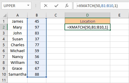
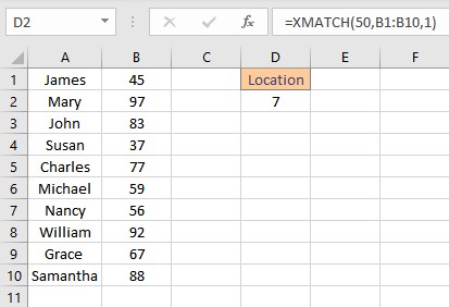
Type =XMATCH(50,B1:B10,1), where 50 is the lookup value, cells B1:B10 contain the table to look up for and 1 is for an exact match of 50 or next larger value.

Press the Enter key to display the result. This displays the location of value 56 as it is the next value larger than 50 which is not present in the range.

Note: This function is available only in Office 365.

Conclusion

In this article, we learned about some of the lookup and reference functions in Excel.

Lookup and Reference Functions in Excel – Part IV