When there are a number of columns with numerical data, say the price details of a few products sold on different days, for instance, it’s a common practice for anyone to want to know how much has been sold in terms of quantity & revenue. So, in this article, we are going to explore the different ways to add a Total Row at the bottom of the data.
- Using the Keyboard Shortcut
- Using the Formulas Tab
- Using SUM Formula
We would be trying to add the quantity and price details of the below dataset using each of the above listed methods.
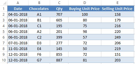
1. Using the Keyboard Shortcut
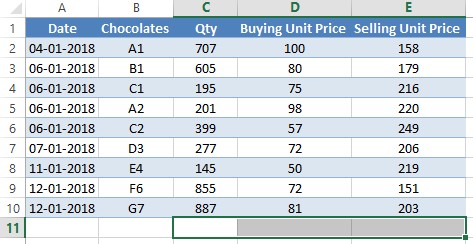
In this data, the totalling is to be done at row 11, just below the columns C, D, E which contains the numerical data. To get things started, select cells from C11 to E11 as shown below,

This can be done by clicking on cell C11 and dragging the mouse till it reaches cell E11. For those who are having a hard time dragging the mouse, the navigation keys come to the rescue!
After clicking on C11, press the SHIFT key on your keyboard & don’t lift the finger off while doing the next operation. Hit the right arrow key (→) until the selection reaches the cell E11.
Once done press the following keys one after the other on your keyboard,
ALT, “+” (PLUS)
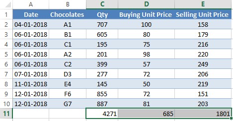
One must focus on making sure that the ALT key is pressed & without lifting that finger, the + (PLUS) key is then pressed. Once it is done, the cells will be populated with the total figure of each of the columns as shown below,

2. Using the Formulas Tab
This is for those who have a hard time remembering the keyboard shortcuts or would like to have a plan-B to add the total row. Selecting the required cells at the bottom of the dataset remains the same as stated in the previous method.
Once done, click on the Formulas Tab as shown in the below image,
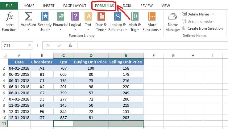
Now, look for the Autosum command within the Formulas tab.
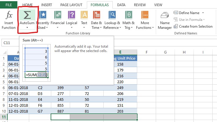
Click on the Ʃ (Summation) symbol as highlighted in the above image & at once the total sum of the columns would appear in each cell selected at their very bottom.
3. Using SUM Formula
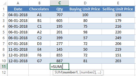
We need not select the cells at the bottom of the columns with the numerical data in here as needed for the previous 2 methods. But we click on cell C11 to get things started.
Double click on the cell and type =SUM( within as shown in the below image.
Once done, select all the numerical entries in the column above.
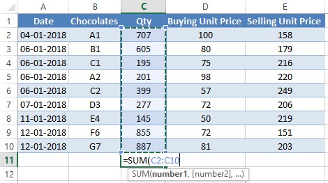
When you see something similar to the selection in the above image, it’s time to close the bracket which was opened right after we typed the word SUM.
Hit ENTER!
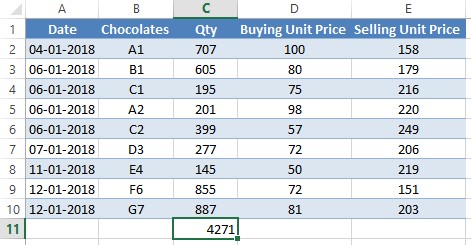
The total figure for all the entries of column C appears. Copy this cell and paste it on the cells D11 and E11 next to it.
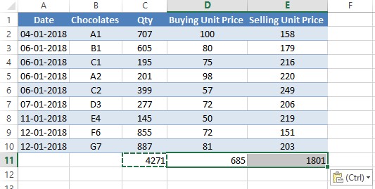
It is now evident, that the total is summed up at the bottom of the entries in the columns D & E too.
Conclusion
Now we’ve covered 2 different ways to add a row with the sum total for a given dataset. Do check this article which covers how to multiply in MS Excel. For more such tricks and tips for using MS Excel, do watch out our space, QuickExcel. Cheers!
