Using a spreadsheet is all about working with numbers and in this article we are going to look into how to carry out one such arithmetic operation using MS Excel.
Enter DIVISION!
In this article, we are going to look into an example where we have the details of the products purchased on different dates along with the total quantity and total price paid for each item.
Hope that the story has written itself out here, where one gets to wonder, ‘How much is the price per unit of each item?’

Now, let’s get on with the task of computing the price per unit of each item with the above data & the method which we are going to put in use goes by the name, The Operand Method.
Also read: How to Add in Excel? [Easy Guide]
Division Using Operators in Excel
Similar to all the formulae constructed in MS Excel, the one which uses the operand too starts with an equal to sign “=” as shown below.

Click on the numerator, which in this case is going to be the entries under the column Total Price. So, we click on cell T2 (Which reminds me of the Terminator movie).
Now hit the ‘/’ slash key on the keyboard so that it gets included in the cell as shown in the below image.

The slash (/) is called the division operand which is used to carry out the arithmetic operation of division in Excel. Similar to the conventional practice, here too we would be placing the operand in between two variables. In this case, that would the Total Price on the numerator and the Qty on the denominator.
Now that the slash is included, we select the cell to fill in the denominator by clicking on cell S2 as shown in the below image.

Press ENTER key and voila! The Total Price of 30 gets divided by the Quantity of 2 and the resulting number 15 is displayed under the Unit Price column of the Product Chips.

Now is the time that this formula gets deployed across the other products as well. Click back on cell U2 and copy the formula in the cell by pressing CTRL+C.

When a dotted line rotates around the cell, similar to the legendary SNAKE game in an old Nokia phone, it means that the contents of the cell are copied & are ready to be pasted elsewhere.
Once done, select the cells U3 and U4 as shown in the below image.

Press CTRL+V to paste the formula into the selected cells. The Unit Price for the Biscuits and the Chocolates would appear in no time.

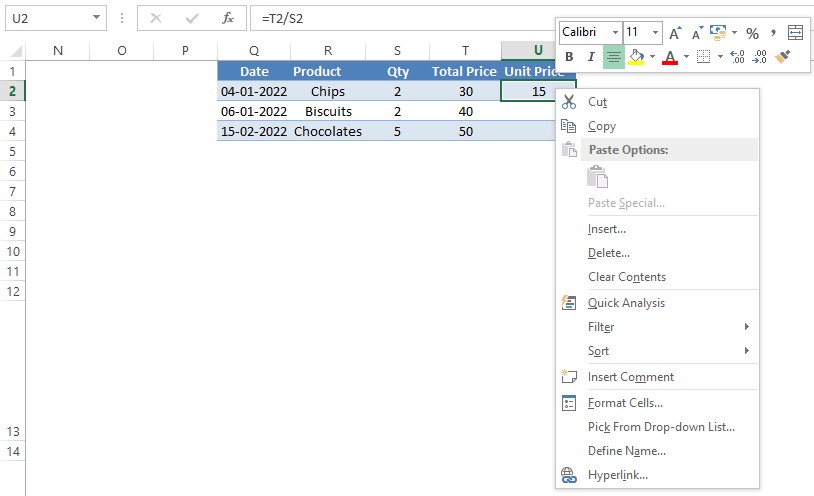
The copying & pasting can also be done using an old school mouse right-click, rather than a keyboard shortcut for those who do not fancy the latter.
Upon right-clicking, the selected cell whose formula is to be copied, the following list of options would appear.

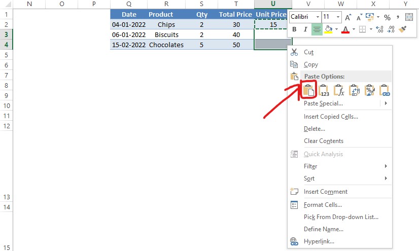
Click on Copy in the list of options & then select the cells into which the copied formula is to be pasted.

After selecting the cells, right click using the mouse anywhere within the selected region & again a list of options to choose from would appear. This time click the Paste icon as shown in the below image.

The formula gets applied and the results would be displayed in a jiffy!

So now we have come across not only how to construct a formula to divide using an operand, but also to copy and paste it to the other cells as well.
Conclusion
Hope the article was informative. To know how to multiply using MS Excel, do have a look at this article. QuickExcel has numerous other articles too which could help you with that one thing that you’re trying to do with MS Excel right now. Ciao!
