In this article, we’ll learn how to perform a T-Test in Excel. Excel offers enough options and features to make our statistical data calculation superfast and time-saving. So, using the statistical data we can perform the T-Test in Excel in a few minutes.
What is a T-Test?
A T-test is one of the hypothesis tests for assuming the means and finding out the significant difference between the given groups. In simple terms, it is the mean calculation of the respected two groups to check out the statistically significant difference between them.
Using the T-test function we will be able to compare the given two samples to find out the core difference between them. From this, we will be able to conclude whether the given samples are of the same composition or significant or not.
Types of T-Test in Excel
Let’s now go over the types of T-Tests that you can perform!
1. One-Sample T-Test
The T-Test has a one-sided critical area of distribution.
2. Two-Sample T-Test
The T-Test has two-sided critical areas of distribution.
3. Independent T-Test
The T-Test is used for comparing the two independent groups through which the statistical significance can be extracted.
How to perform a T-Test in Excel?
Finding the statistical probability of the students using the t-Test function is quite easy. By adopting the simple steps one can easily find out the significance between the given two sets of groups.
The T-Test function helps to determine whether the given two sets of population/ group are significant or not. For this, we have to take an example of two groups like the height of the boys and girls.
1. Find an Average
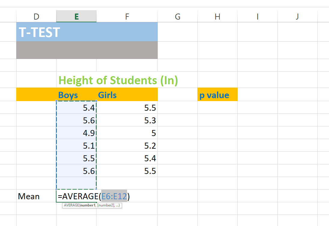
Create the two sets of the group, here we have created the height of some boys in one column and girls height in another column.
Find the Mean of each Group, to find the mean using the formula, =AVERAGE(E6:E12). Here I mean you have to select all the values to find the average
As in our example,
Boys, =AVERAGE(E6:E12)
For Girls, =AVERAGE(F6:F11)
2. Finding the P-Value
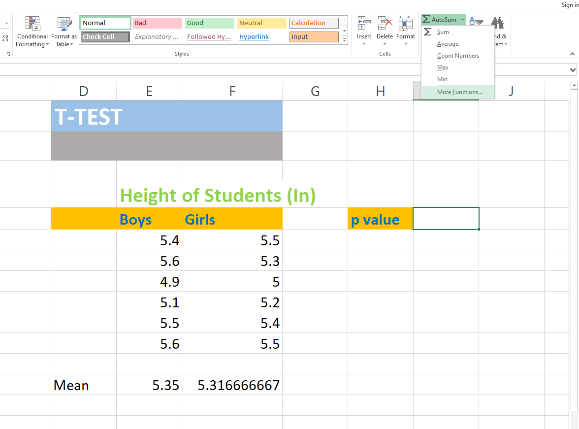
- Click on the function menu and then More Functions.
- Find and select the Statistical as a category of the functions.
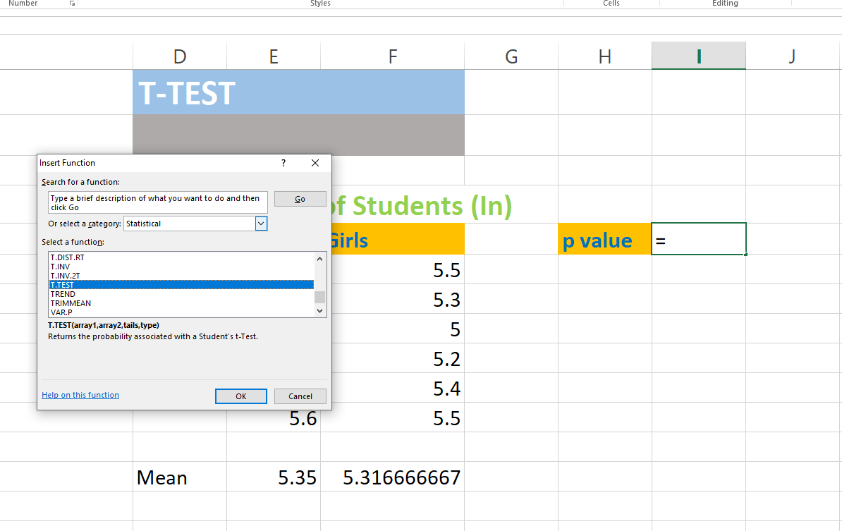
- Select the T.TEST from the ‘Select a function’ under Statistical category.
3. Selecting the Arguments
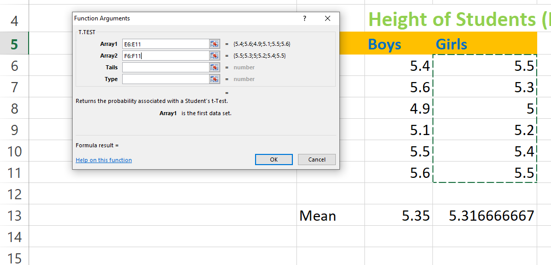
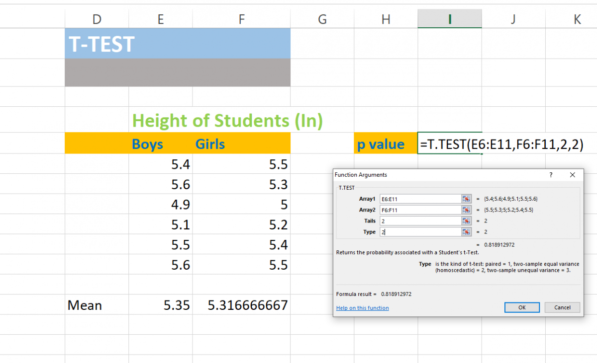
In Arrary1 select all cells of the column. Here in Arrary1, we’ve selected the Boys values from E6 to E11. It’s the 1st data set to be selected.
Select the Arrary2 for Girls from F6 to F11. It means here we have to enter the second or another data set to compare with 1st data set/column.
4. Choosing the Number of Distributions
Enter 1 or 2 as per the nature of the distribution of your data. Basically, if there are cells having the same or equal value then we can use 1, if not then we can use 2 instead of 1.
Now specify the number of tails distribution. For one tail distribution enter 1 and enter 2 for two-tailed distribution. Here we want to work on 2 tail distributions. So, we enter 2.
5. Choosing the Right Parameters in Type
Enter the number 1, 2, or 3 as per the t-test that is intended to be performed.
For Paired use 1, use 2 for Two-sample equal variance and 3 for Two-sample unequal variance.
To perform Two samples equal variance t-test we’ve to enter the value 2 in type. So, enter 2.
6. Finalizing the P-Value
After entering the information on Function Arguments hit OK. Here we get the p-value of 0.81891.
Here we got the p-value greater than 0.5 which determines there isn’t a significant difference between the height of boys’ and girls’.
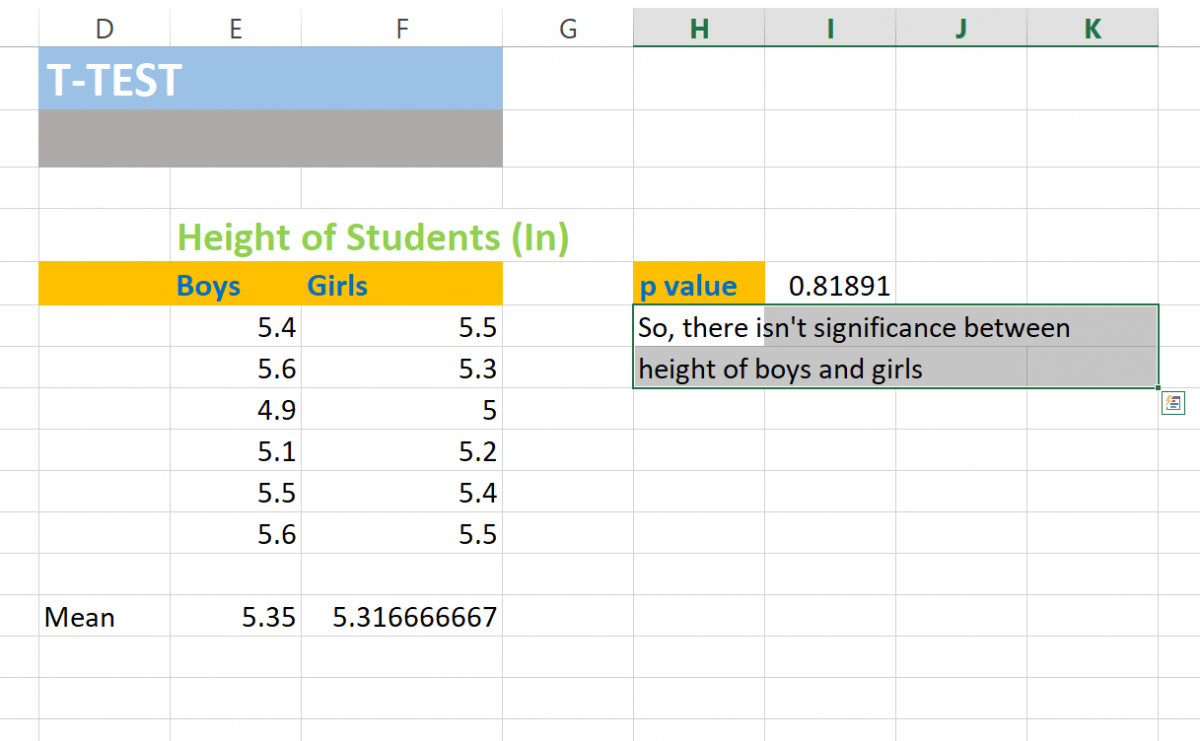
(Remember, the p-value below 0.500 is to be treated as the significant difference and above than it is treated as it’s not a significant difference between the given two datasheets.)
Conclusion
That’s it for the tutorial. Hope you have learned well about t-tests and how to do t-test in excel. Stay tuned for more such tutorials on Excel.
