Tips to Use Excel’s Filter Tool for Faster Data Analysis

Welcome to this incredible tutorial on the Filter tool in Microsoft Excel for quicker and improved data analysis. By the end of this tutorial, you understand how the Filters help you filter data in different ways. Make sure to read till the end to learn in detail about the filter tool.

Let’s get cracking!

Getting started: Filter Tool in Excel

Let’s begin to learn the filter tool from scratch!

1. Opening the filter tool

The filter tool in Excel is located under the Data tab in the Sort & Filter section.

Filter shortcut key– CTRL+Shift+L

You can use this shortcut on a data range to automatically apply filters on the range without going to the Data tab.

Or, you can right-click on a value in a data range, click Filter, and apply a custom filter.

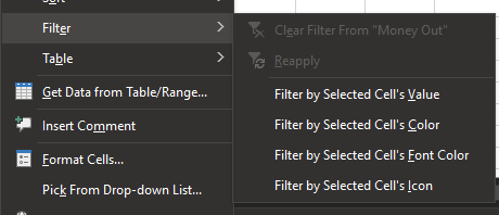
Let’s learn more about the filter tool with an example.

Here’s is a sample mailing list.

Let’s apply filters to sort out specific information from this range.

For example, we’re interested in sorting out customers based in England only. There are multiple ways you can do this using the filter tool.

Method 1

Click on a cell with England in the State column.
Right-click on it and click Filter.
Choose Filter by Selected Cell’s Value.

You will see that the mailing displays contacts living in England only.

Method 2

Here’s a long method to achieve this.

Press CTRL+Shift+L to apply filters to the range.
Or, click on Filter in the Data tab.
Click on the down arrow near State to open filter options.
Uncheck Select All to uncheck everything.
Check England.
Click OK.

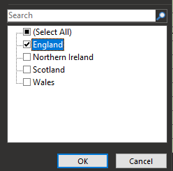
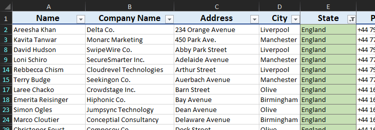
You can see that only contacts based in England are displayed.

Note that the unfiltered data is hidden and not deleted. You can push the down arrow button to edit the filter. Press CTRL+Shift+L to remove all filters from the table range.

2. Filtering multiple columns or data

Now, let us filter out contacts who are specifically based in Liverpool, England.

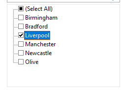
Pull down on the State column and deselect all states.
Check England and click OK.
Pull the arrow down on the City column and deselect all cities.
Check Liverpool and click OK.

You can see those contacts living specifically in Liverpool, England have been filtered.

You can also right-click on Liverpool and England one by one and select the Filter by Selected Cell’s Value option.

3. Filtering data alphabetically

If you want to filter the contact list alphabetically, you can easily do it using the filter tool. You can apply alphabetical filtering to any column you like.

Let’s sort and filter the mailing list in an A-to-Z alphabetical order of contact names. Here are the steps.

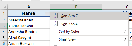
Pull the arrow down near the Name column.
Click on Sort A to Z.

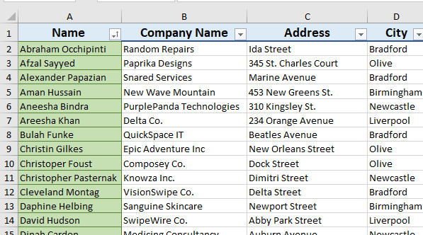
You can see that the contact names are arranged in alphabetical order.

4. Sorting data in ascending or descending orders

If you want to sort any numerical data in ascending or descending orders, you can easily do it using the filter tool.

Let’s sort the contact numbers in descending order as an example. Here are the steps.

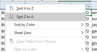
Pull the arrow down near the Phone column.
Click on Sort Z to A.

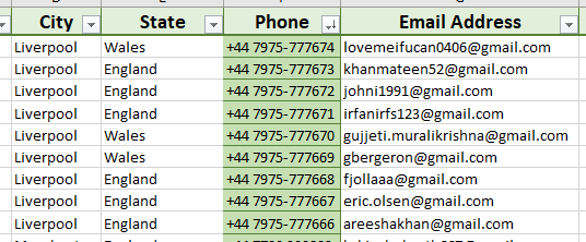
You can see that the phone numbers are arranged in descending order. Similarly, you can do the same if you want to arrange the data in ascending order.

5. Filtering custom values

You can type in a custom value from the range that you want to be filtered by using a wild card in the filter options. Let’s learn it with an example.

For instance, let’s sort out all addresses with the word “Avenue” in them.

Method 1

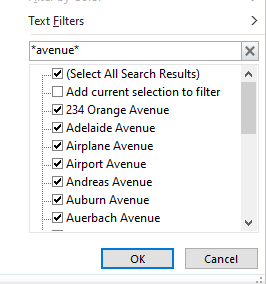
Open the filter options for the Address column.
Deselect all filters by unchecking Select All.
Click in the search box under Text Filters.
Type *avenue* in the box.
Click OK.

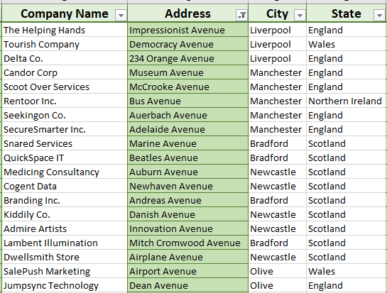
You will notice that all addresses with the word “avenue” are sorted out by the tool.

Method 2

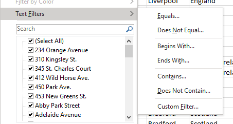
Open the filter options for the Address column.
Click on Text Filters.
Click Contains.
Choose And.
Enter the word “Avenue”
Hit OK.

6. Filter by color

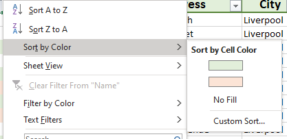
If you have colored some cells in the data range, and want to sort only those cells, you can do this using the filter tool. Here are the steps.

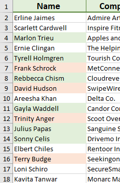
Notice that some cells are colored in light red and some in light green.

Let’s filter out the red colors cells using the filter tool.

Pull down on the filter arrow for the column you want to filter by color.
Click Filter by Color.
Select the cell color you wish to filter.

You can see those cells with red color have been filtered out.

You can also sort cells with red color at the top by clicking the Sort by Color option.

7. Filter by time or date

To filter data by time and date, follow the steps below.

Open the filter options.
Click Date Filters.
Choose a filter you like. For example, Next month.

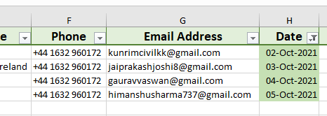
You can see that the range is displaying data for the next month, that is, October.

You can filter a custom date by clicking the Between option in the date filter.

Conclusion

This article was a detailed tutorial on the filter tool in Microsoft Excel. We learned about a variety of filter options and their application to real data. You can play around with the different options based on your needs and easily filter out the crucial data from a range. Stay tuned for more interesting tutorials like this!