IRR in Excel - How to Calculate the Internal Rate of Return in Excel?

In this article, we’ll learn how to calculate IRR in Excel. Internal Rate of Return (IRR) is a popular budgeting metric of capital used to estimate the return of potential investment.

Also read: ROI in Excel – How to Calculate ROI in Excel

Formula to calculate IRR

IRR or Internal rate of return is a method of calculating an investment’s rate of return. As by the name, it only takes into consideration internal factors and parameters of an organization/firm/investment in calculation and excludes external factors, such as market demand, market sentiments, inflation, the cost of capital.

Mathematical Formula:

IRR can be calculated by equating the Net Present Value (NPV) equation equal to zero (0) and solving for the rate of return (IRR).

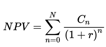
IRR formula in Excel — IRR formula (equate to 0)

where:

N: total number of periods
NPV: Net Present Value
n: a non-negative integer
: cash flow
: internal rate of return

Formula to Calculate IRR in Excel

The formula to calculate IRR in Excel returns the internal rate of return for a series of cash flows.

=IRR (values, [guess])

The excel function uses two arguments:

Values (required argument) – An array of values, representing the series of cash flows. Cash flows include investment and net income values. Values can be a reference to a range of cells containing values.
[Guess] (optional argument) – This is a number guessed by the user that is close to the expected internal rate of return (as there can be two solutions for the internal rate of return). If skipped, the function will take a default value of 0.1 (=10%).

Steps to calculate IRR in Excel

Let’s get into calculating the IRR in Excel with the help of an existing dataset.

Step 1: Input the Data

Enter the relevant data in correct formatting, for which you want to calculate IRR.

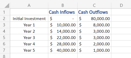
Here, in our example, we are calculating the IRR of a company, started five years ago. We have Cash Outflows and Cash Inflows data with us. You may notice that the ‘Initial Investment’ adjacent cell of Cash Inflows is empty, the reason being, that our example company was set up (started) at that time with an initial investment of $80,000, hence No Cash Inflows.

Sample data of cash inflows and outflows in excel — Sample data of cash inflows and outflows to calculate IRR

Step 2: Calculate the Net Flow

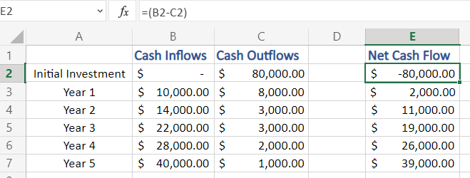
Now, we need to calculate the Net Cash Flow.

Net Cash Flow = Cash Inflows – Cash Outflows

Here, in our example, it would be found using (B2-C2)

Apply the same formula to all the cells of the ‘Net Cash Flow’ column. (You may encounter both positive and negative values, as Net Cash Flow of a company can be either)

calculate net cash flow in excel — Calculate net cash flow

Step 3: Apply the IRR formula

To apply the IRR formula, select a cell for output
Then type in:

=IRR(

Select, all the data values, for which you want to find the IRR from the Net Cash Flow column (include all positive and negative values), in our example all values from E2:E7

Close the formula bracket and hit Enter to apply the formula.

=IRR(E2:E7)

Applying IRR formula in Excel — Applying IRR formula

You must have got the final output for IRR (Internal Rate of Return) in the output cell

IRR in Excel, not precise — IRR (not precise)

But, the IRR that we have calculated is not precise and may lead to erroneous assumptions and calculations when dealing financial data.
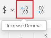
To make Internal Rate of Return (IRR) precise we, need to increase the Decimal Value precision in our output cell.
To do so, select Home in your Home tab and click on Increase Decimal (2 or 3 times, as per decimal places required)

increase decimal precision in excel — increase decimal precision

Hence, we get our final and precise result for Internal Rate of Return (IRR):

Conclusion

That’s It! Hope you have learned well – What is Internal Rate of Return (IRR), and how to calculate IRR in Excel.