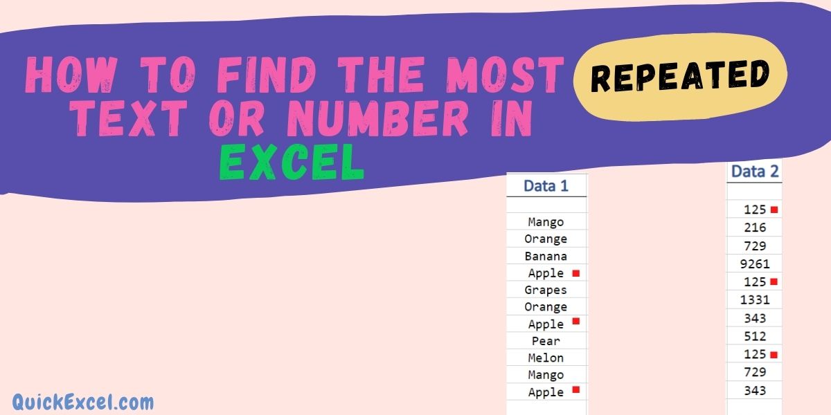
There are multiple instances that you would require to find the most repeated or maximum occurring Text or Number in your Excel worksheet.
Follow this step-by-step tutorial, to learn how to use these functions to find the most frequently occurring or repeated text or number in Excel.
Also read: Calculating Ratio, Frequency, and Percentage in Excel – Quick and Easy Guide
Steps to find the most repeated text or number
To count the most frequently occurring text or number in Excel: We do this by using a combination of the INDEX, MODE, and MATCH functions.
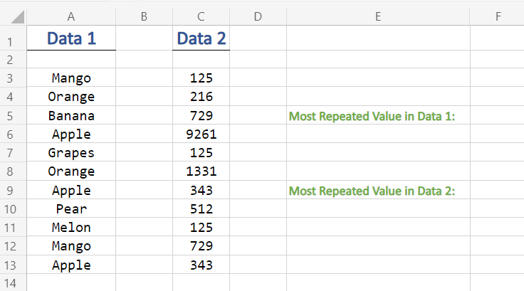
Step 1. Enter the data
- Input a relevant data set in your Excel worksheet, in which you want to find the most frequently occurring text or number. Sample data values are shown below in two different columns for checking for text and numbers individually.
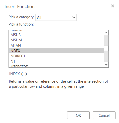
Step 2. Insert Index function
- Insert a function in the output cell, by inserting the INDEX function or typing in:
=INDEX(
in the above function bar
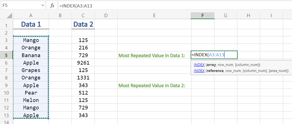
- Now, Select all the data cell values by dragging, in which you want to analyze for most repeated values
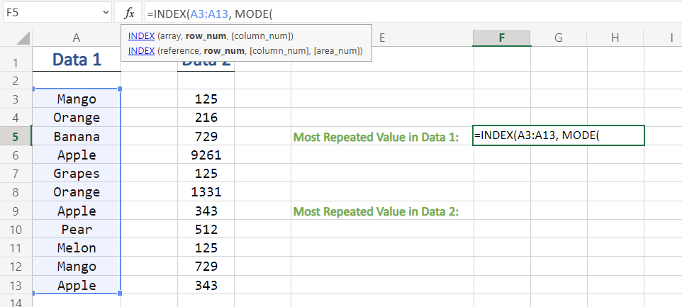
here in our example, we are performing the operation on Data 1 column. Hence, at first, we are selecting the ‘Data 1’ column. Here, selecting A3:A13
Step 3. Insert Mode function
- After selecting the data cell values, put a comma in the function bar
- After the comma, insert MODE function by typing ,MODE( after the selection
=INDEX(A3:A13, MODE(
Step 4. Insert Match function
- Now, again insert another function in the bar by typing in MATCH(
=INDEX(A3:A13, MODE(MATCH(

Step 5. Putting Values and Final Output
- After inputting of various functions, its time to enter data values,
- Select the same data values of the same column as done in Step 2
=INDEX(A3:A13, MODE(MATCH(A3:A13
- Put a comma(,) and yet again select the same data values.
=INDEX(A3:A13, MODE(MATCH(A3:A13,A3:A13
- Now, input a comma followed by a zero (0).
- Close the bracket three times and hit Enter to apply the formula.

=INDEX(A3:A13, MODE(MATCH(A3:A13,A3:A13,0)))
Now, you will be presented with the final output for the Most Repeated Value, here in the column of ‘Data 1’
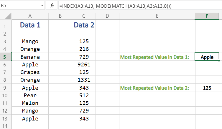
We have used the same steps to find the most repeated value in the ‘Data 2’ column for numbers.
Conclusion
That’s It! We hope you learned and enjoyed this lesson on how to find the most repeated text and numbers in your Excel worksheet, stay tuned and we’ll be back soon with another awesome Excel tutorial at QuickExcel!
