A Pivot Table is a magical data analysis tool that will help you handle these extremely large data sets effortlessly and in the shortest time possible.
With Pivot tables you can easily manage, re-order, categorize and classify large databases into fewer relevant data sets.
Steps to create a pivot table from scratch
Let us proceed to learn how to make a perfect Pivot Table from scratch with supporting images, step-by-step.
1. Open your data sheet
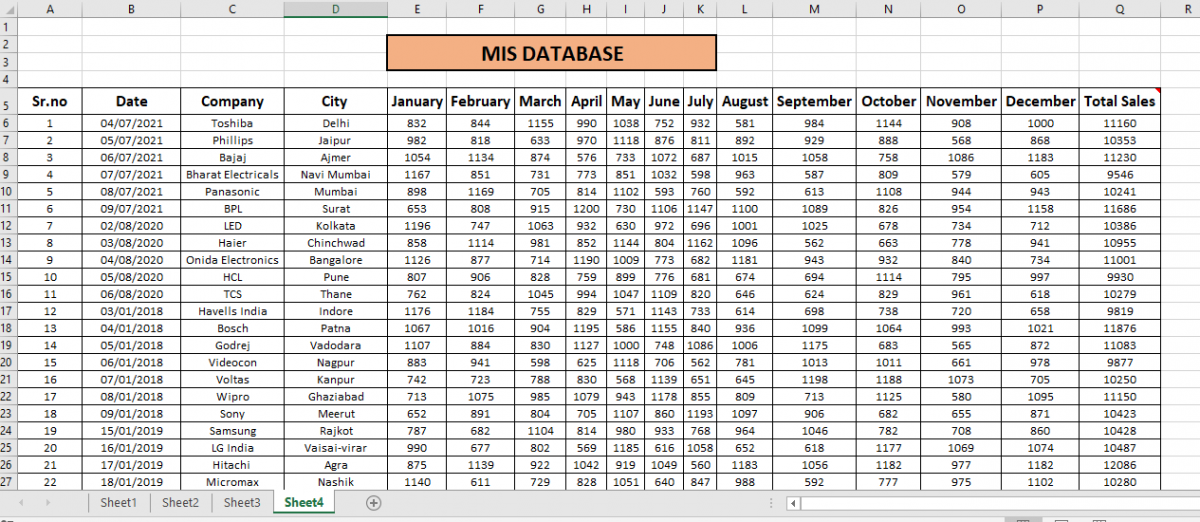
First, let us take an example of a fairly large database here-

For instance, assume that you’re working for an ecommerce company and it has this sales data of electronic companies in different Indian cities.
There are sales data for 12 months and a column named ‘Total Sales’ which denotes the sum of sales of all months of every company.
Now, you are interested in finding out the sales data of a specific company, for example, Panasonic for the months of May, September and December.
But looks like it is quite a difficult task to hide all unwanted figures that are not required for a while. Fortunately, it is possible with Pivot Tables!
2. Select with the data range
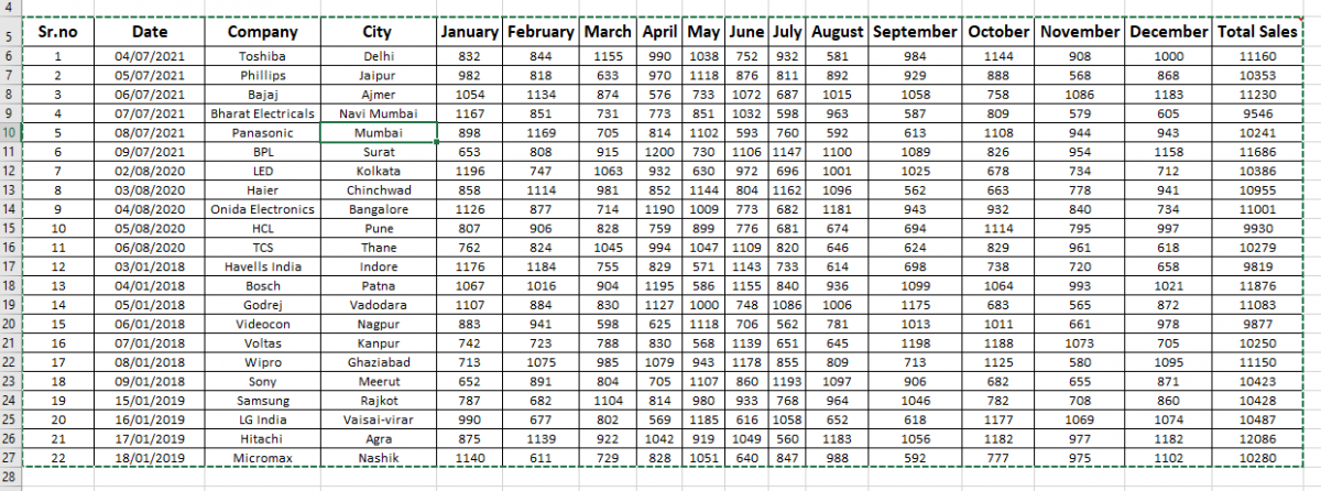
First, select a cell within the database and go to the ‘Insert’ tab above. Click Pivot Table, which opens a window called ‘Create Pivot Table’ which automatically selects your database’s table range.
If not, click on the Table/range box and select the entire database range like this-

Before clicking OK, you have the options to create the Pivot Table in a new Sheet or somewhere in the existing sheet.
You can choose the ‘Existing Worksheet’ option and select a blank cell where you want your Pivot Table to begin from (below or besides the database), as it will be more convenient for you.
Or you can simply choose the ‘New Worksheet’ option if you want the table in a fresh blank sheet. Now, press OK to create the table.
3. Setup the pivot table
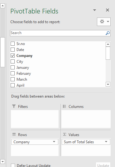
You can now see Pivot Table Fields options at the right-hand side of the screen. This field enables you to sort and view only those fields and data figures from your database that is relevant to your study.

In our example, we want to find out the sales data of the company Panasonic for the months of May, September and December.
From the check box, select ‘Company’, ‘May’, ‘September’ and ‘December’. This will be the result-

Now select the pull-down button besides Row labels, uncheck ‘Select All’ and check ‘Panasonic’.

You now have a 3-month data sorted for Panasonic with the help of Pivot Tables. You can even filter and sort data in ascending or descending orders and much more.
Conclusion
This was all about creating a basic Pivot Table from scratch for a large database and to achieve organizational objectives quickly by saving time. If you have any doubts, drop your questions below in the comments and we will be pleased to help you out!
