Even the simplest of the operations turns out to be exhaustive when it tends to be run for umpteen iterations. The same can be told for addition too.
But worry not, for MS Excel has got other ways to get things done swiftly rather than sluggishly carrying them out like a handheld calculator. In this article, we are going to look into the details of adding multiple cells in MS Excel using each of the below techniques.
- The Operand Way
- The SUM Formula
- By AUTOSUM
- By Paste Special
Following is the dataset that shall be used for demonstrating it throughout.

Also read: How to Merge Data From Two Columns in MS Excel?
The Operand Way:
Synonymous with the way we are used to adding numbers back in school, this is the simplest of the options available but is not advisable for computing a chunk of data. Reading further, you will know why.
As always with any formula, we start with an equals sign (=) at the bottom of the column where the marks are listed & select each cell followed by including a plus sign (+) after each cell as shown below.
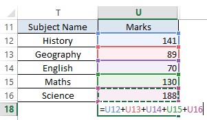
Hit ENTER & the total shall appear.
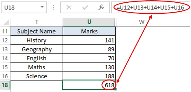
The sheer efforts taken to select each cell with the number & place a plus sign in between them is what makes this technique the least preferred.
The SUM Formula:
This is a sleek way to get multiple cells added in a blink of an eye. The formula is started in the same way with an equals sign (=), followed by typing SUM as shown below.
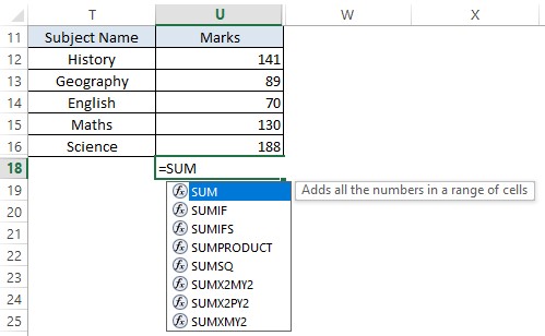
Unlike the previous technique, one has to include the cells only within a pair of round parentheses due to the inherent feature of MS Excel requiring to do so. Include an opening round parenthesis following SUM & left click on the very first cell (U12) in the list of numbers to be added as shown below.
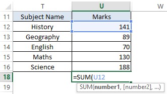
Now without taking the finger off the left mouse button, drag the cursor all the way down to U16 at the bottom of the list and close the round parenthesis as shown below.
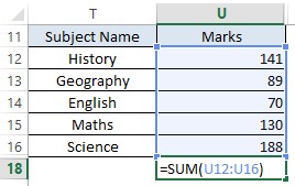
Hit ENTER & the total figure appears!
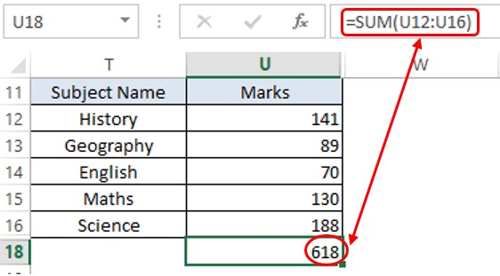
By AUTOSUM:
This is the fastest option available to add multiple cells in Excel, but the only pre-requisite here is that the cell in which the total is to be calculated should be right at the bottom of the list of numbers.
AUTOSUM isn’t compatible to carry out its function if the cell in which the result of addition is to be displayed and the list of numbers to be added are separated from each other. Also, it adds numbers only vertically (i.e) along the column & not across the rows.
Click at the very bottom of the list of numbers & use the keyboard shortcut ALT + PLUS (+).
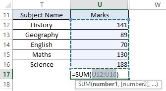
All the cells above the cell in which the formula is constructed shall be selected as shown above. Hit ENTER & the total shall be displayed.

By Paste Special:
Suppose one has to add 5 marks say ‘for good handwriting’ across all these subjects then the same can be done using a rather infamous & a bit contradicting technique. This ain’t a formula per se, but can be used very well to add a given number across the selected cells.
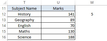
Copy the cell W12 which contains the 5 marks that need to be added. Now select all the cells containing the marks of the subjects as shown below.
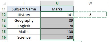
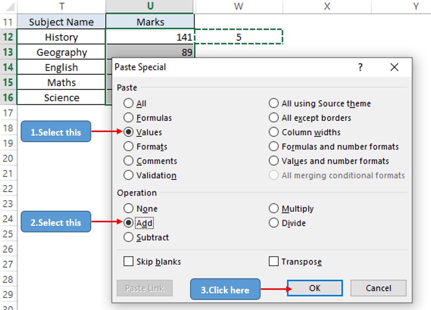
Use the keyboard shortcut CTRL+ALT+V & the following pop-up appears. Select the Values & Add option as shown below.
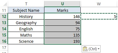
All the subject marks would have now been increased by 5.
Conclusion:
Now that we are concluding this article, hope it has given you the much-needed clarity on adding multiple cells in MS Excel. Here’s an article which elaborates on how to copy a formula in MS Excel. There are also other cool articles in QuickExcel that will help you catch up with ever-evolving trends. Cheers!
