Acts of mischief – that’s one word which comes into our mind when the spreadsheets we get have some ‘hidden’ agenda. Though it may be unintentional, it gets us into a grave problem when certain entries go hiding, especially when there is a formula involved. It makes us lose our precious time, leaving us scratching our heads on what went possibly wrong.
Also read: How to Hide Cells in MS Excel?
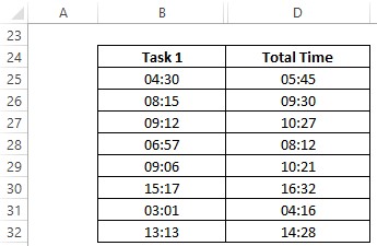
One might adopt all the troubleshooting techniques that one knows of, only to find out that the culprit lies not in the formula but hidden between the rows or the columns. Consider the following example in which column C is hidden between columns B & D.

In this article, we shall set out to explore how to unhide the hidden cells in the above data using each of the below techniques.
- The Conventional Right Click
- The Accelerator Way
Method 1 – The Conventional Right Click:
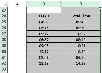
The mouse would be the weapon of choice in this technique, facilitating us with the oldest trick in the book – the RIGHT CLICK! One shall get started by selecting both the columns between which a column lies hidden. In this case, one shall select columns B to D as shown below.

The selection can be done by hovering the cursor & pulling it from wherever it is to the portion where the column names are indicated by letters. It is in this region that the cursor changes from a normal mouse pointer to a thick black arrow facing downwards as shown in the below image.

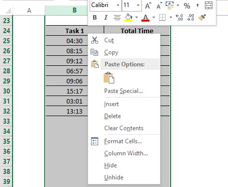
Now one shall click right on the top of the column at the letter ‘B’ & drag the cursor towards the right to column ‘D’. Once done, right-click anywhere within the selected region as done in the image below.

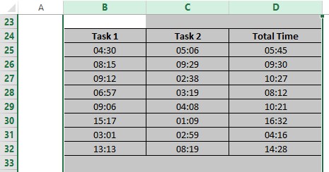
There shall be a right-click menu appearing with a list of options. Choose the Unhide option in the list & the hidden culprits would appear right in front of your eyes as shown below.

Method 2 – The Accelerator Way:
This technique is way simpler & relies more on the keyboard for successful execution. The first step of selecting the cells to unhide hidden cells remains the same as that of the previous method.

Once done, hit the ALT key on the keyboard followed by the letter keys O, C & U.
ALT + O + C + U
All these keys are to be pressed one after the other & not simultaneously. Doing the latter would only render this technique non-functional. It is also to be noted that the succeeding key is to be pressed after lifting the finger off the preceding key – to put in simple words, not similar to what one does with CTRL+C for copying or CTRL+V for pasting.
The moment the last key in the sequence, the letter key ‘U’ is hit, the hidden cells appear in a blink of an eye!

Both the techniques serve the purpose when the cells are also hidden horizontally along the rows, rather than vertically along the columns as given in the above examples.
Summary
Now we have reached the end of this article detailing how to unhide cells in MS Excel. Hope it has provided you with the sufficient information that you were looking for. Here is something that elaborates on How to Move a Column in MS Excel? Go on & read it to know further. There are also numerous other articles in QuickExcel that can come in handy for those who would like to constantly upgrade themselves in MS Excel. Cheers!
