One can’t be successful if one has got to do everything by oneself. Similarly, it would be an insurmountable task if one has to type in all that is needed to carry out a computation in MS Excel. So, in this article let’s explore the different ways to link the cells and their corresponding implications.
MS Excel has an inherent feature that automatically updates the cell references when any formula is applied across a selection of cells. But, not always this comes in handy. At times, we would be needing to restrict the reference given in a formula to one particular cell alone & would not want that to be changing across the cells where the formula is being applied.
In order to satisfy such a requirement, there are multiple ways in which the cells linked to a formula can be referred to. These are listed as follows,
- Conventional Referencing
- Absolute Referencing
- Relative Referencing
Before getting into details of each of these methods, one has got to understand how cells are being named in MS Excel to master the art of referencing.
Each cell is named by an alphabet indicating the column in which it is present, followed by a number which indicates the row in which it is present. This cell name is also known as the address of the cell.
So, when someone tells A1, it means that they’re referring to the cell which is positioned where column A & row 1 intersects as shown below.
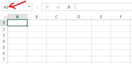
The box indicated by an arrow in the above image is known as the address bar & wherever the cursor clicks on the spreadsheet, this section shall display the address of that cell.
Method 1 – Conventional Referencing
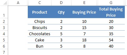
In this method, there would not be any special precautions taken while linking the cells within the formula. This is the default cell reference which would be followed by MS Excel. The below image depicts a typical formula constructed using this type of reference.

The results of the above formula are given below.
Method 2 – Absolute Referencing
One has got to introduce a dollar ($) sign between both the alphabet & the number. Now one can wonder when would this be applicable? So here’s an example!
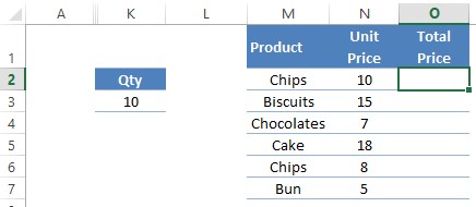
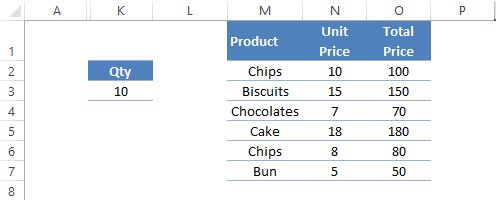
In the above data set, the quantity is the same for all the items. So, the formula cannot be constructed in accordance with the previous method since that would use a different cell reference for each cell in which it is deployed.
We restrict the formula to refer only to the cell K3 which has the quantity by adding a dollar ($) sign before the alphabet, K and the number, 3.
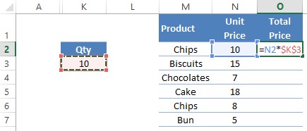
Hit Enter & copy the formula to paste it through the rest of the cells in column O and one could see that the formula in all the cells refers to K3 alone.

Here’s the result of the above table after deploying the formula to all the cells in column O.
Method 3 – Relative Referencing
Take this example below where we would be referring to the same column D for the quantity details to calculate the entries for column H – Total Selling Price.

When we copy these formulae as-is & paste them into column H, the following happens.

So, it is clear that the cell references have been shifted one cell to the right while the copied formulae are pasted in column H. To tackle this, we shall include a dollar sign only before the alphabet D as shown below & copy that formula to cells of column H.

Following are the results of the above formulae.

Similarly in cases where the row reference is to remain the same, then the dollar ($) sign is placed only before the number & not the alphabet.
Conclusion
We have reached the end of this article. Do have a look at this article, to know how to view formulae in MS Excel. Nevertheless, QuickExcel has numerous other articles, which would be of great help to you when it comes to understanding the nuances of working with MS Excel. Cheers!
