What-if analysis is an important and highly advantageous tool in Microsoft Excel that contains three tools under it namely Scenario Manager, Goal Seek, and Data Table. These tools are highly useful and handy in business management and analysis and can help in achieving important business objectives.
We will learn each of these tools in-depth to get a complete understanding of the What-if Analysis tool in Excel.
What-if Analysis tools and using them in Excel
Let’s get started with this detailed step-by-step guide to using and learning Scenario Manager, Goal Seek, and Data table tool under What-if analysis.
1. Steps to use Scenario Manager in Excel
Scenario Manager is a tool under what-if analysis in Excel that can be used for comparing real values with assumed and forecasted values for a product or item.
For example, this tool can be used in comparing the current cost with a probable minimum and maximum cost of an item.
Let’s take this instance forward and learn how the Scenario Manager tool can help us out. To begin with, we take a current cost breakdown of an item of an imaginary company for the month of January.
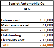
2. Comparing costs using Scenario Manager
We will now create two scenarios with estimated minimum cost and maximum cost, then compare these two with the current cost, with the Scenario Manager.
- Go to the Data tab.
- Under the Forecast group.
- Pull-down on What-if Analysis.
- Click on Scenario Manager.
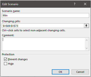
- Once the Scenario Manager window opens, click Add.
- In the Add Scenario window, name your scenario in Scenario Name that is suitable to you. Here, we will name our first scenario as “Min” because we are creating a minimum cost scenario.
- Backspace comments if you do not wish to see them.
- Check Prevent Changes to protect the summary from being manipulated.
- Hit OK to proceed to the next step.
You will now see a window named Scenario Values which shows all values you selected from the table.
Simply change the values to the estimated/forecasted minimum costs for the item.
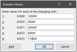
Now that we also want to add the estimated maximum costs, we will click Add instead of OK.
- Name your scenario as “Max” this time.
- Select the current costs from the table again.
- Hit OK to proceed.
- Enter the maximum estimated costs for the item.
- Hit OK.
You now see all newly created scenarios listed in the Scenario Manager.
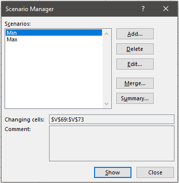
- Click Summary to view the Scenario Summary.
- In the Scenario Summary window, select the cell with a total cost in the data table and hit OK to continue.
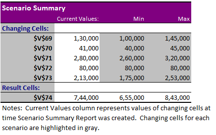
You can see that a scenario summary has been created in a new sheet named Scenario Summary, showcasing current costs and estimated minimum and maximum costs.
3. Steps to use Goal Seek in Excel
The Goal Seek tool can be found under What-if analysis in the Data tab in Excel. This tool is used to estimate a value required to achieve a given specific goal or target.
Learn about the Goal Seek tool in detail here: How to use Goal Seek in Excel?
For instance, you are a teacher in a school, and it runs examinations for 6 subjects. But examinations of only 5 subjects were given by all students due to a weather change and sudden floods.
You are now supposed to reckon a predicted mark for students in the 6th subject. Let’s see how Goal Seek can help us out.
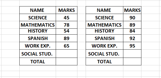
There are two types of students here; an average and a nerd. You have to predict a figure for a mark lost based on the marks obtained in the other 5 subjects, for the 6th subject.
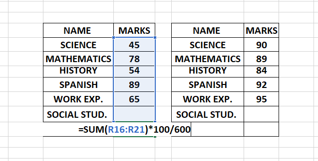
- To begin with, we will first find a total percentage for all cells with and without marks for both students.
- Also, find a percentage for 5 subjects for both students to understand their performances in the attempted tests solely (exclude the blank cell).
- This figure will help you determine a number in Goal seek settings to set as the goal TOTAL to be achieved to predict a mark for the 6th subject.
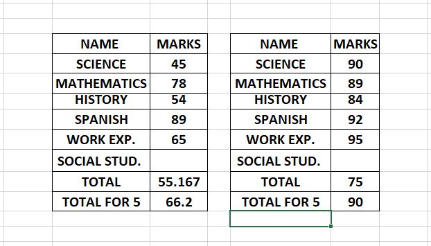
- Go to the Data tab, under the Forecast section, pull-down on What-if Analysis.
- Select Goal Seek which will now open a new window called Goal Seek.
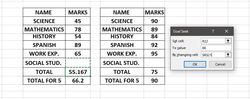
- In the Set cell box, select the cell with total percentage for 6 subjects.
- In To value, enter the total percentage you found for 5 subjects.
- By changing cells, select the empty cell without marks i.e., the marks of the 6th subject.
- Hit OK and you now have the mark for the 6th subject.
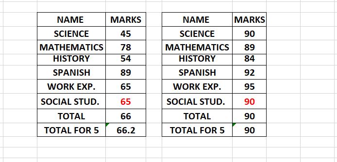
This is how Goal Seek in Excel can help you predict or find out missing or estimated figures in a dataset.
4. Steps to use Data Table in Excel
Data Table is a beneficial tool that helps you determine multiple answers to a specific problem. You can use data tables to achieve a variety of objectives with the right knowledge.
Let’s take a simple example to help you understand what Data Table is and how to use it in Excel.
We have a product with a total quantity of 40,000 units in stock priced at $20 per unit. The total revenue is $800,000 at this price. We are interested in finding out the revenues at different prices and at varying numbers of units.
This is where the Data Table tool can come in handy. Let’s learn to create a complete dataset that displays changing revenue rates at changing prices and quantities of a product in Excel.
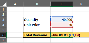
- First, calculate the total revenue by multiplying 40,000 units by $20.
- Remember to use a formula to calculate the revenue for creating a data table. You can either use the PRODUCT formula to multiply or write 40,000 and 20 in two different cells and multiplying them like this- =cell1*cell2.
- select a cell below this table, type ‘’=’’ and select the cell with calculated profit and hit ENTER.
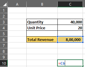
- The calculated revenue should be displayed in that cell.
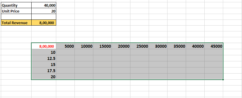
- We now horizontally type some quantity values in the increment of 5,000 units each.
- Type the varying prices in the increment of $0.50, vertically.
- Now, select the table area to let the data table put revenue values at these prices and quantities.
This is how your table should be structured and selected for the data table to function.
- Once the table is selected, go to the Data tab.
- Under the Forecast section, pull-down on What-if Analysis.
- Select Data Table which will now open a new window called Data Table.
- In the Row Input Cell, select the quantity that is, 40,000 in C3.
- In the Column Input Cell, select the price $20 that is, C4.
- Click OK to apply.

You can find that you’ve got revenue calculations at different prices and quantities for the same product. So, you now know that the revenue is $150,000 if you sell 15,000 units at $10.
Recommended read: How to Stop Excel from Rounding?
Conclusion
This article was all about the What-if Analysis tool in Excel. Comment your queries below and get answered!
References: Microsoft
