2 Easy Ways to Transpose Data in Excel

If you want to transpose data in Excel to convert rows to columns or the inverse, then Excel has already made it easier for you to do it.

Transposing vertical data to horizontal data or horizontal data to vertical data can be done using two methods. This article is a step-by-step guide to transpose data in excel.

Recommended read: How to group rows and columns in Excel?

Steps to transpose in Excel

Let’s get started with the steps to transpose data in Excel. There are two ways to transpose data in Excel, one, transpose with paste special, and two, using the TRANSPOSE function.

Transposing data with Paste Special

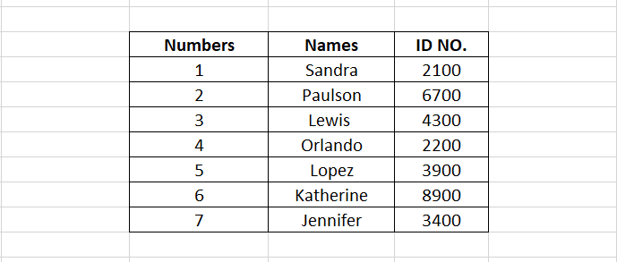
First, we take an example of a vertical database to further transpose this data-

Sample Database Transpose Data in Excel — Sample Database

Select the entire database to transpose.
Press CTRL + C on your keyboard or select the Copy option in the Home tab to copy the database.
Select a blank cell in an empty area in the worksheet to paste the database.
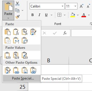
Pull down on Paste in Home tab under Clipboard section.
Select Paste Special at the bottom.

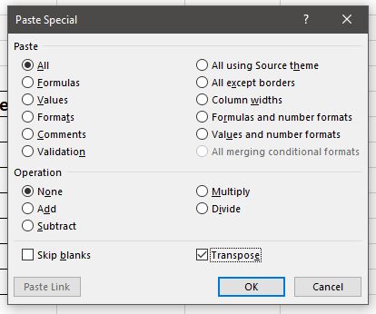
A new window opens showing Paste Special options –

Check Transpose at the bottom.
Hit OK.

Your data is now transposed. This is how it should look like-

Transposed Database Transpose Data in Excel — Transposed Database

Transposing data with TRANSPOSE formula

If you don’t want to transpose your database using Paste Special options, then you can use the TRANSPOSE function in Excel to do the same for you, but it is quite a lengthy process.

Here is how you can do it-

We take the same database to transpose using TRANSPOSE formula–

Select the same number of blank cells that are taken by your database, but horizontally, like this-

Horizontal Replica of Vertical Database Transpose Data in Excel — Horizontal Replica of Vertical Database

Without clicking anywhere else, start typing the TRANSPOSE formula i.e., =TRANSPOSE(
Press Tab on your keyboard or double-click on the formula when it is suggested by Excel, to use the formula.
Select the database after typing =TRANSPOSE( when asked for the array.
Close brackets after selecting the database, but don’t press ENTER yet!

Transpose Array Selection Transpose Data in Excel — Transpose Array Selection

Press CTRL + SHIFT + ENTER to apply the TRANSPOSE function with the array formula. This is because we have selected more than one cell to apply a formula and ending a function with an array formula (CTRL + SHIFT + ENTER) will enable the function to be applied on more than one cell.
Do NOT press ENTER right away after completing the TRANSPOSE function or you will see a #VALUE! an error like this-

#VALUE! Error Transpose Data in Excel — #VALUE! Error

After applying the function with array formula, your data will now be transposed, like this-

Conclusion

This was a detailed and step-by-step guide on two ways to transpose your data in Excel. If you have any doubts regarding any of the steps mentioned above, drop your queries below and we will answer them!