Hundreds of thousands of entries recorded one below the other – a typical description of a massive spreadsheet constructed in MS Excel. Spreadsheets like these would take a lot of time to go through & one would be in dire need of something that could summarize the entries in a particular column. Let’s consider a tabulation of Sales data, for instance, the first thing that might pop in anyone’s mind while looking at it would be, how much has been sold in total?
In this article, we would be covering the different ways of totalling the entries of a column in the below dataset.
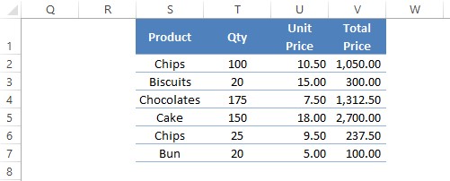
- SUM using Cell Range
- SUM using Column Name
Method 1 – SUM using Cell Range:
The name of the formula itself is self-explanatory for the functionality that it provides. So, having that sorted out, we shall now look into how to put that into use by trying to total the entries under the Qty. column.
Also read: How to Add in Excel? [Easy Guide]
We shall get things started by clicking on the first blank cell at the bottom of the column as shown below & type =SUM( within.
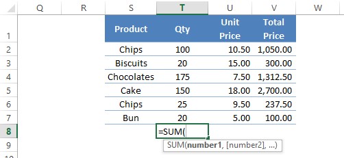
Once done, click on the very first entry on the column which would be cell T2 & select all the entries to the very bottom, till T7 as shown in the below image.
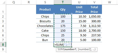
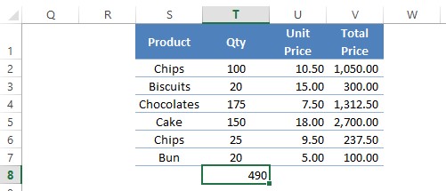
Include a closing bracket ‘ ) ’, hit ENTER & the total of all the entries shall be displayed in that cell.
Method 2 – SUM using Column Name:
There always lies a potential window of error when one has to choose the range of cells to be totaled while constructing a formula. Also, when the workbook is made accessible to a number of users, there is no guarantee that the range given in the formula remains the same. Nevertheless, there is a way around to counter these shortcomings.
Behold!
The COLUMN NAMING!
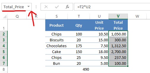
What this does is help us put a name of our choice over a selected range of cells so that whenever we want to use a particular range of cells in a formula, we might not select the entire set of cells manually but just type in the name which we gave to them!
The execution too would be fairly simple as would be stated below.
We shall get started by selecting the range of cells which we want to total, the column Total Price for instance.
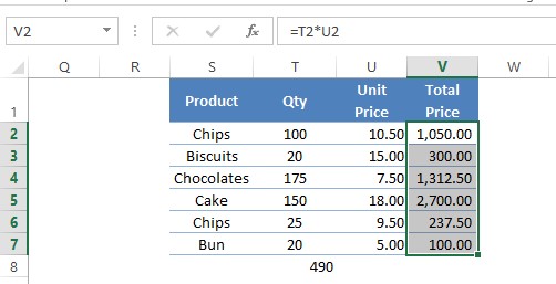
Once done, click on the cell address box as shown below & type the name of your choice.
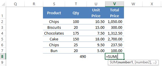
Now we trace resume to the very first step of the previous method in which we type the formula, =SUM( within the first blank cell at the bottom of the column as shown below.
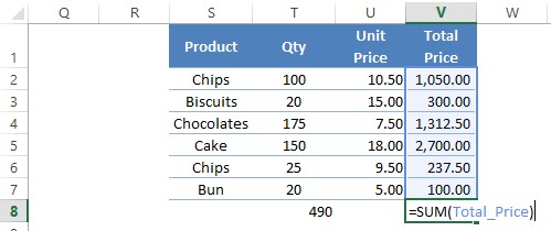
Here’s the cool part, where we need to type in the name we gave rather than selecting the cells. Type a few letters of the name & Excel shall suggest the name available for selection as shown in the below image.
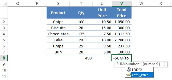
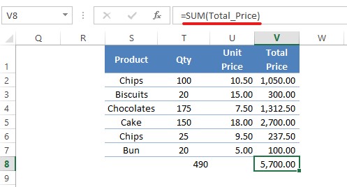
Click on the named range & include a closing bracket ‘ ) ‘ to complete the formula. Hit ENTER & the total calculated shall be displayed within cell V8.
Conclusion:
Now we have reached the end of this article about totaling a column in MS Excel. QuickExcel has numerous other articles too that can come in handy for those who are looking to explore the lengths & breadth of MS Excel. Here’s one which elaborates on how to insert a column in MS Excel. Cheers!
